In the dynamic world of finance, understanding and effectively managing risk within a portfolio of assets is paramount to achieving financial objectives and safeguarding investments. Portfolio risk assessment involves evaluating and quantifying the various risks associated with the assets held in a portfolio. In this article, we explore the key concepts, methodologies, and considerations involved in assessing and quantifying risk within a portfolio.
Diversification as a Portfolio Risk Mitigation Strategy
One of the foundational principles of portfolio risk assessment is diversification. Diversifying a portfolio involves selecting a mix of assets with varying risk-return profiles. The goal is to reduce the impact of adverse events on the overall portfolio by spreading risk across different asset classes, industries, and geographical regions. Diversification is based on the principle that not all assets will react in the same way to market fluctuations or economic events.
Read More about Beta and Systematic Risk here……….
Types of Portfolio Risk
- Systematic Risk: This type of risk, also known as market risk, is inherent in the overall market and affects all assets to some degree. Systematic risk is caused by macroeconomic factors, political events, interest rate changes, and other market-wide influences. Measuring systematic risk often involves assessing an asset’s beta, which quantifies its sensitivity to market movements.
- Unsystematic Risk: Also called specific risk, unsystematic risk is unique to individual assets or specific sectors. It can arise from company-specific factors such as management decisions, competitive pressures, or supply chain issues. Unsystematic risk can be mitigated through diversification, as the impact on one asset may not affect others.
Key Steps in Portfolio Risk Assessment
- Asset Selection: The first step is to carefully select assets for the portfolio. Investors must consider their risk tolerance, investment horizon, and financial goals. Assets are chosen based on their expected returns, risk profiles, and correlation with existing portfolio holdings.
- Risk Metrics: Various risk metrics and ratios are used to assess and quantify risk. These include beta, standard deviation, and Value at Risk (VaR). Beta helps measure systematic risk, standard deviation assesses overall portfolio volatility, and VaR estimates potential loss at a specified confidence level.
- Correlation Analysis: Understanding how different assets within the portfolio are correlated is essential. Negative correlations can help reduce risk, while high positive correlations may increase it.
- Scenario Analysis: Investors perform scenario analysis to evaluate how the portfolio might perform under various economic conditions or unexpected events. Stress testing is a component of scenario analysis that assesses portfolio resilience under extreme market conditions.
import numpy as np
import pandas as pd
import yfinance as yf
import matplotlib.pyplot as plt
from scipy.optimize import minimize

# Download historical stock data
tickers = ['AAPL', 'MSFT', 'GOOGL', 'AMZN', 'TSLA']
data = yf.download(tickers, start='2020-01-01', end='2024-01-01')['Adj Close']

# Calculate daily returns
returns = data.pct_change().dropna()

# Define annualization factors
trading_days_per_year = 252

# 1. Equal-Weighted Portfolio
equal_weights = np.array([1/len(tickers)] * len(tickers))
equal_portfolio_return = np.dot(equal_weights, returns.mean()) * trading_days_per_year
equal_portfolio_volatility = np.sqrt(np.dot(equal_weights.T, np.dot(returns.cov() * trading_days_per_year, equal_weights)))
equal_sharpe_ratio = equal_portfolio_return / equal_portfolio_volatility

# 2. Risk Parity Portfolio (Equal Risk Contribution)
def risk_parity_objective(weights, cov_matrix):
    portfolio_variance = np.dot(weights.T, np.dot(cov_matrix, weights))
    marginal_contribution = cov_matrix @ weights
    risk_contribution = weights * marginal_contribution / portfolio_variance
    return np.sum((risk_contribution - portfolio_variance / len(weights)) ** 2)

def risk_parity_portfolio(cov_matrix):
    n_assets = cov_matrix.shape[0]
    init_guess = np.array([1/n_assets] * n_assets)
    bounds = [(0.0, 1.0) for _ in range(n_assets)]
    constraints = {'type': 'eq', 'fun': lambda weights: np.sum(weights) - 1}
    result = minimize(risk_parity_objective, init_guess, args=(cov_matrix,), bounds=bounds, constraints=constraints)
    return result.x

risk_parity_weights = risk_parity_portfolio(returns.cov() * trading_days_per_year)
risk_parity_portfolio_return = np.dot(risk_parity_weights, returns.mean()) * trading_days_per_year
risk_parity_portfolio_volatility = np.sqrt(np.dot(risk_parity_weights.T, np.dot(returns.cov() * trading_days_per_year, risk_parity_weights)))
risk_parity_sharpe_ratio = risk_parity_portfolio_return / risk_parity_portfolio_volatility

# 3. Mean-Variance Optimization (Markowitz Efficient Portfolio)
def portfolio_return(weights, mean_returns):
    return np.dot(weights, mean_returns) * trading_days_per_year

def portfolio_volatility(weights, cov_matrix):
    return np.sqrt(np.dot(weights.T, np.dot(cov_matrix * trading_days_per_year, weights)))

def negative_sharpe_ratio(weights, mean_returns, cov_matrix, risk_free_rate=0.01):
    portfolio_ret = portfolio_return(weights, mean_returns)
    portfolio_vol = portfolio_volatility(weights, cov_matrix)
    return -(portfolio_ret - risk_free_rate) / portfolio_vol

def mean_variance_optimized_portfolio(mean_returns, cov_matrix):
    n_assets = len(mean_returns)
    init_guess = np.array([1/n_assets] * n_assets)
    bounds = [(0, 1) for _ in range(n_assets)]
    constraints = {'type': 'eq', 'fun': lambda weights: np.sum(weights) - 1}
    result = minimize(negative_sharpe_ratio, init_guess, args=(mean_returns, cov_matrix), bounds=bounds, constraints=constraints)
    return result.x

mean_variance_weights = mean_variance_optimized_portfolio(returns.mean(), returns.cov())
mean_variance_portfolio_return = portfolio_return(mean_variance_weights, returns.mean())
mean_variance_portfolio_volatility = portfolio_volatility(mean_variance_weights, returns.cov())
mean_variance_sharpe_ratio = (mean_variance_portfolio_return - 0.01) / mean_variance_portfolio_volatility

# Displaying the results
portfolios = ['Equal-Weighted', 'Risk Parity', 'Mean-Variance Optimized']
returns_list = [equal_portfolio_return, risk_parity_portfolio_return, mean_variance_portfolio_return]
volatility_list = [equal_portfolio_volatility, risk_parity_portfolio_volatility, mean_variance_portfolio_volatility]
sharpe_ratios = [equal_sharpe_ratio, risk_parity_sharpe_ratio, mean_variance_sharpe_ratio]

df_results = pd.DataFrame({
    'Portfolio': portfolios,
    'Return (Annualized)': returns_list,
    'Volatility (Annualized)': volatility_list,
    'Sharpe Ratio': sharpe_ratios
})

print(df_results)

# Plot the results for visualization
fig, ax = plt.subplots(figsize=(10, 6))
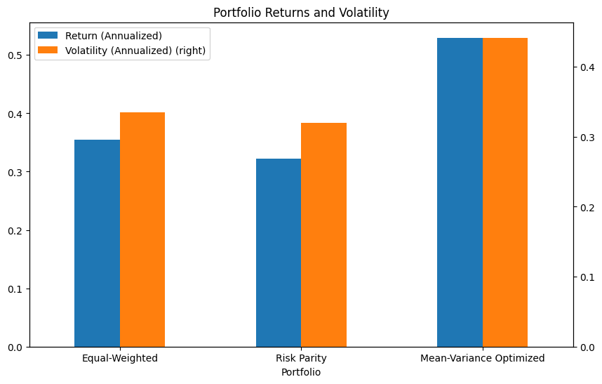
df_results.plot(kind='bar', x='Portfolio', y=['Return (Annualized)', 'Volatility (Annualized)'], ax=ax, secondary_y='Volatility (Annualized)', rot=0)
plt.title('Portfolio Returns and Volatility')
plt.show()
Read more articles on – QuantEdX
Challenges and Considerations for Portfolio Risk Assessment
- Data Quality: The accuracy of risk assessments depends on the quality and relevance of data used for analysis.
- Changing Market Dynamics: Market conditions can change rapidly, and historical data may not always be indicative of future performance.
- Model Assumptions: Many risk assessment models rely on assumptions that may not hold true in all situations. Investors should be aware of these limitations.
Conclusion
Portfolio risk assessment is a fundamental aspect of effective portfolio management. It helps investors make informed decisions, allocate assets in line with their risk tolerance, and prepare for various market scenarios. As financial markets continue to evolve, understanding and mastering portfolio risk assessment remains essential for achieving financial goals while effectively managing the complexities of the investment landscape.