In the world of finance, investors are perpetually seeking the golden balance between maximizing returns and minimizing risk. The Markowitz Model, developed by Nobel laureate Harry Markowitz in 1952, revolutionized modern portfolio optimization theory by introducing the concept of diversification and risk management. At the core of this theory lie two key portfolios: the Minimum Variance Portfolio and the Tangency Portfolio, which form the basis of the Efficient Frontier. In this article, we will explore these essential concepts, provide the mathematical equations behind them, and guide you through their practical implementation using R programming.
For more such Projects in R, Follow us at Github/quantifiedtrader
Understanding the Markowitz Model
The Markowitz Model is built upon the fundamental principle that diversification can lead to portfolio optimization and a more favorable risk-return tradeoff. It introduced the concept of risk as variance, quantifying it in terms of portfolio volatility. Here’s how the key elements of this model work together:
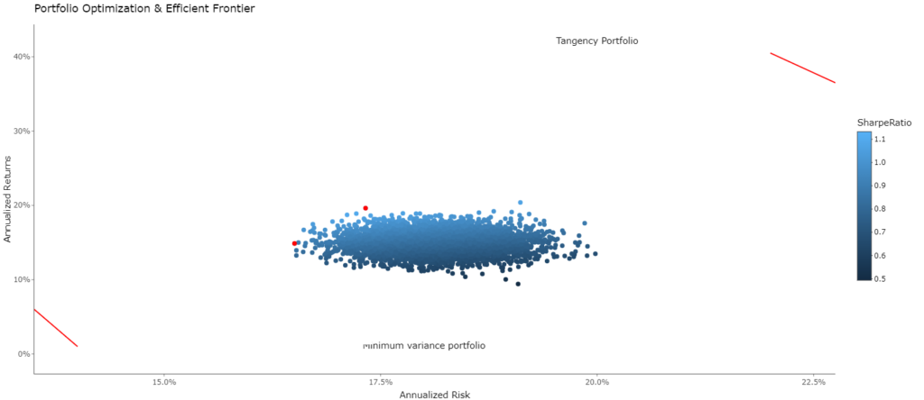
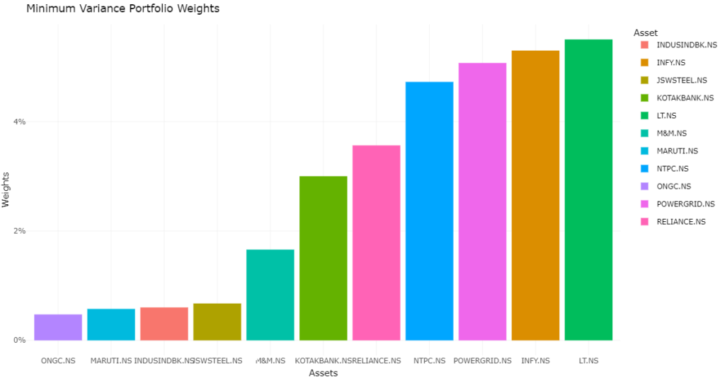
- Minimum Variance Portfolio (MVP): The MVP represents the portfolio with the lowest possible risk for a given level of return. It is constructed by optimizing the weights of assets in the portfolio to minimize its variance, hence the name “minimum variance.”
- Tangency Portfolio: The Tangency Portfolio is the optimal portfolio for investors who consider both risk and return. It is the point at which the Capital Market Line (CML), representing the risk-return tradeoff, is tangent to the Efficient Frontier. The Tangency Portfolio maximizes the Sharpe Ratio, which measures the excess return earned per unit of risk.
- Efficient Frontier: The Efficient Frontier is a graph that shows all possible portfolios an investor can construct, each with a unique risk-return profile. Portfolios lying on the Efficient Frontier are considered “efficient” because they offer the highest return for a given level of risk or the lowest risk for a given level of return.
Equations Behind Markowitz’s Model
To calculate the Minimum Variance Portfolio and Tangency Portfolio, you need the following equations:
Minimum Variance Portfolio (MVP):
- Portfolio Variance:
σ^2(p) = w^T * Σ * w - Where
wis the vector of asset weights, andΣis the covariance matrix.
Tangency Portfolio:
- Expected Portfolio Return:
μ(p) = w^T * μ - Portfolio Variance:
σ^2(p) = w^T * Σ * w - Where
wis the vector of asset weights,μis the vector of expected returns, andΣis the covariance matrix.
Practical Implementation with R
Now, let’s put the theory into practice with R programming. The provided code demonstrates how to calculate these portfolios and visualize the Efficient Frontier using historical stock data.
library(quantmod)
library(dplyr)
library(tidyr)
library(PerformanceAnalytics)
library(quantmod)
library(ggplot2)
library(plotly)

# Define the list of stock tickers
tick <- c('RELIANCE.NS', 'SBIN.NS', 'ICICIBANK.NS', 'CIPLA.NS', 'INFY.NS',
          'M&M.NS', 'DRREDDY.NS', 'TATAMOTORS.NS', 'BHEL.NS', 'TCS.NS',
          'HCLTECH.NS', 'HEROMOTOCO.NS', 'HINDALCO.NS', 'HINDUNILVR.NS',
          'BAJAJ-AUTO.NS', 'BPCL.NS', 'COALINDIA.NS', 'JSWSTEEL.NS', 'KOTAKBANK.NS',
          'LT.NS', 'MARUTI.NS', 'NTPC.NS', 'ONGC.NS', 'POWERGRID.NS', 'SUNPHARMA.NS',
          'TITAN.NS', 'UPL.NS', 'ULTRACEMCO.NS', 'WIPRO.NS', 'ADANIPORTS.NS',
          'ASIANPAINT.NS', 'AXISBANK.NS', 'BAJAJFINSV.NS', 'BAJFINANCE.NS',
          'BHARTIARTL.NS', 'GRASIM.NS', 'HDFCBANK.NS', 'INDUSINDBK.NS')

# Get historical price data for all stocks
price_data <- tq_get(tick,
                     from = '2014-01-01',
                     to = '2020-12-20',
                     get = 'stock.prices')

# Calculate daily log returns for all stocks
log_ret_tidy <- price_data %>%
  group_by(symbol) %>%
  tq_transmute(select = adjusted,
               mutate_fun = periodReturn,
               period = 'daily',
               col_rename = 'ret',
               type = 'log')

# Convert log returns to xts format
log_ret_xts <- log_ret_tidy %>%
  spread(symbol, value = ret) %>%
  tk_xts()

# Calculate mean returns for all stocks
mean_ret <- colMeans(log_ret_xts)
print(round(mean_ret, 5))

# Calculate covariance matrix
cov_mat <- cov(log_ret_xts) * 252
print(round(cov_mat, 4))

# Generate random portfolio weights
set.seed(123)  # For reproducibility
wts <- runif(n = length(tick))
print(wts)

# Normalize portfolio weights
wts <- wts / sum(wts)
print(wts)

# Calculate portfolio returns
port_returns <- (sum(wts * mean_ret) + 1)^252 - 1

# Calculate portfolio risk
port_risk <- sqrt(t(wts) %*% (cov_mat %*% wts))
print(port_risk)

# Calculate Sharpe ratio
sharpe_ratio <- port_returns / port_risk
print(sharpe_ratio)

# Number of portfolios to simulate
num_port <- 5000

# Creating matrices and vectors to store portfolio metrics
all_wts <- matrix(nrow = num_port, ncol = length(tick))
port_returns <- vector('numeric', length = num_port)
port_risk <- vector('numeric', length = num_port)
sharpe_ratio <- vector('numeric', length = num_port)

# Simulate random portfolios
for (i in seq_along(port_returns)) {
  wts <- runif(length(tick))
  wts <- wts / sum(wts)
  all_wts[i, ] <- wts

  # Portfolio returns
  port_ret <- sum(wts * mean_ret)
  port_ret <- ((port_ret + 1)^252) - 1
  port_returns[i] <- port_ret

  # Portfolio risk
  port_sd <- sqrt(t(wts) %*% (cov_mat %*% wts))
  port_risk[i] <- port_sd

  # Portfolio Sharpe Ratios (assuming 0% Risk-free rate)
  sr <- port_ret / port_sd
  sharpe_ratio[i] <- sr
}

# Store portfolio metrics in a tibble
portfolio_values <- tibble(Return = port_returns,
                           Risk = port_risk,
                           SharpeRatio = sharpe_ratio)

# Convert matrix to tibble and change column names
all_wts <- tk_tbl(all_wts)
colnames(all_wts) <- colnames(log_ret_xts)

# Combine portfolio metrics with weights
portfolio_values <- tk_tbl(cbind(all_wts, portfolio_values))

# Find minimum variance and maximum Sharpe ratio portfolios
min_var <- portfolio_values[which.min(portfolio_values$Risk), ]
max_sr <- portfolio_values[which.max(portfolio_values$SharpeRatio), ]

# Plot minimum variance portfolio weights
p_min_var <- min_var %>%
  gather(RELIANCE.NS:INDUSINDBK.NS, key = Asset,
         value = Weights) %>%
  mutate(Asset = as.factor(Asset)) %>%
  ggplot(aes(x = fct_reorder(Asset, Weights), y = Weights, fill = Asset)) +
  geom_bar(stat = 'identity') +
  theme_minimal() +
  labs(x = 'Assets', y = 'Weights', title = "Minimum Variance Portfolio Weights") +
  scale_y_continuous(labels = scales::percent)

# Plot maximum Sharpe ratio portfolio weights
p_max_sr <- max_sr %>%
  gather(RELIANCE.NS:INDUSINDBK.NS, key = Asset,
         value = Weights) %>%
  mutate(Asset = as.factor(Asset)) %>%
  ggplot(aes(x = fct_reorder(Asset, Weights), y = Weights, fill = Asset)) +
  geom_bar(stat = 'identity') +
  theme_minimal() +
  labs(x = 'Assets', y = 'Weights', title = "Tangency Portfolio Weights") +
  scale_y_continuous(labels = scales::percent)

# Plot efficient frontier
p_eff_frontier <- portfolio_values %>%
  ggplot(aes(x = Risk, y = Return, color = SharpeRatio)) +
  ylim(0, 0.20) +
  geom_point() +
  theme_classic() +
  scale_y_continuous(labels = scales::percent) +
  scale_x_continuous(labels = scales::percent) +
  labs(x = 'Annualized Risk',
       y = 'Annualized Returns',
       title = "Portfolio Optimization & Efficient Frontier") +
  geom_point(aes(x = Risk, y = Return), data = min_var, color = 'red') +
  geom_point(aes(x = Risk, y = Return), data = max_sr, color = 'red') +
  annotate('text', x = 0.20, y = 0.42, label = "Tangency Portfolio") +
  annotate('text', x = 0.18, y = 0.01, label = "Minimum variance portfolio") +
  annotate(geom = 'segment', x = 0.14, xend = 0.135, y = 0.01,
           yend = 0.06, color = 'red', arrow = arrow(type = "open")) +
  annotate(geom = 'segment', x = 0.22, xend = 0.2275, y = 0.405,
           yend = 0.365, color = 'red', arrow = arrow(type = "open"))

# Convert ggplot plots to plotly for interactivity
p_min_var_plotly <- ggplotly(p_min_var)
p_max_sr_plotly <- ggplotly(p_max_sr)
p_eff_frontier_plotly <- ggplotly(p_eff_frontier)

# Display the interactive plots
p_min_var_plotly
p_max_sr_plotly
p_eff_frontier_plotly
This code utilizes the quantmod and ggplot2 libraries to retrieve historical stock data, calculate portfolio returns and risk, and visualize the results. You can adapt this code to your own dataset and customize it as needed.
Conclusion
The Markowitz Model, with its Minimum Variance and Tangency Portfolios, remains a cornerstone of modern portfolio theory. By understanding and implementing these concepts, investors can better navigate the complex world of finance, optimizing their portfolios to achieve their financial goals while managing risk effectively. Whether you’re a seasoned investor or a beginner, Markowitz’s ideas continue to offer valuable insights into the art of portfolio management.
FAQs
Why is diversification important in the Markowitz Model?
Diversification spreads risk across different assets, reducing the overall portfolio risk. Markowitz’s model quantifies this diversification benefit and helps investors optimize their portfolios accordingly.
What is the Sharpe Ratio, and why is it significant?
The Sharpe Ratio measures the risk-adjusted return of a portfolio. It’s essential because it helps investors evaluate whether the excess return they earn is worth the additional risk taken.
Can I apply the Markowitz Model to any asset class?
Yes, you can apply the Markowitz Model to any set of assets, including stocks, bonds, real estate, or a combination of asset classes. However, accurate historical data and covariance estimates are crucial for its effectiveness.