Monte Carlo simulations are a class of computational algorithms with the power to unlock solutions for problems that have a probabilistic interpretation. They are incredibly versatile and widely used in various fields, including finance, physics, engineering, and more. In this article, we’ll take a deep dive into Monte Carlo simulations, with a focus on their application in simulating stock price dynamics, particularly using the Geometric Brownian Motion model.
A Brief History
The Monte Carlo method takes its name from the Monte Carlo Casino in Monaco. This name was chosen as a code name for the method during the Manhattan Project, a top-secret research and development project during World War II. Scientists working on the project needed to simulate the behavior of neutrons in nuclear reactions, and they used randomness to tackle this problem.
Monte Carlo Simulations: An Overview
The central idea behind Monte Carlo simulations is to generate a vast number of sample paths or possible scenarios. These scenarios are often projected over a specific time horizon, which is divided into discrete time steps. This process of discretization is vital for approximating continuous-time phenomena, especially in domains like financial modeling, where the pricing of assets occurs in continuous time.
Simulating Stock Price Dynamics with Geometric Brownian Motion
One of the essential applications of Monte Carlo simulations in finance is simulating stock prices. Financial markets are notoriously unpredictable, and understanding potential price movements is crucial for various financial instruments, including options. The randomness in stock price movements is elegantly captured by stochastic differential equations (SDEs).
Geometric Brownian Motion (GBM)
Geometric Brownian Motion (GBM) is a fundamental model used to simulate stock price dynamics. It’s defined by a stochastic differential equation, and the primary components are as follows:
- S: Stock price
- μ: Drift coefficient, representing the average return over a given period or the instantaneous expected return
- σ: Diffusion coefficient, indicating the level of volatility in the drift
- Wt: Brownian Motion, which accounts for random fluctuations in the stock price
The GBM model is ideal for stocks but not for bond prices, which often exhibit long-term reversion to their face value.
The GBM Equation
The GBM model can be represented by the following stochastic differential equation (SDE) in LaTeX:
dS = \mu S dt + \sigma S dW_t
In this equation, μ is the drift, σ is the volatility, S is the stock price, dt is the small time increment, and dWt is the Brownian motion.
Simulating Stock Prices
To simulate stock prices using GBM, we employ a recursive formula that relies on standard normal random variables. The formula is as follows:
S_{t+1} = S_t \cdot e^{\left(\mu - \frac{\sigma^2}{2}\right)\Delta t + \sigma \sqrt{\Delta t} \cdot Z_t}Here, Zt is a standard normal random variable, and Δt is the time increment. This recursive approach is possible because the increments of Wt are independent and normally distributed.
In the progression of this article, we conducted several essential steps in the context of financial simulations:
Step 1: We acquired stock price data and computed simple returns.
Step 2: Subsequently, we segregated the data into training and test sets. From the training set, we calculated the mean (drift or mu) and standard deviation (diffusion or sigma) of the returns. These coefficients proved vital for subsequent simulations.
Step 3: Furthermore, we introduced key parameters:
- T: Denoting the forecasting horizon, representing the number of days in the test set.
- steps: Representing the number of time increments within the forecasting horizon.
- S_0: Indicating the initial price, derived from the last observation in the training set.
- num_simulations: Reflecting the number of simulated paths.
Monte Carlo simulations are grounded in a process known as discretization. This approach entails dividing the continuous pricing of financial assets into discrete intervals. Thus, it’s imperative to specify both the forecasting horizon and the number of time increments to align with this discretization.
Step 4: Here, we embarked on defining the simulation function, a best practice for tackling such problems. Within this function, we established the time increment (dt) and the Brownian increments (dW). The matrix of increments, organized as num_simulations x steps, elucidates individual sample paths. Subsequently, we computed the Brownian paths (W) through cumulative summation (np.cumsum) over the rows. To form the matrix of time steps (time_steps), we employed np.linspace to generate evenly spaced values across the simulation’s time horizon. We then adjusted the shape of this array using np.broadcast_to. Ultimately, the closed-form formula was harnessed to compute the stock price at each time point. The initial value was subsequently inserted into the first position of each row.
import numpy as np
import pandas as pd
import yfinance as yf
import matplotlib.pyplot as plt
# Define the asset symbol
asset_symbol = 'SBIN.NS'
# Download historical data for the asset
data = yf.download(tickers=asset_symbol, start="2022-01-01", end="2023-01-01", interval='1d')
# Extract adjusted closing prices and calculate daily returns
adjusted_close_prices = data['Adj Close']
returns = adjusted_close_prices.pct_change().dropna()
# Plot the distribution of returns
returns.plot(figsize=(15, 6), title="Returns Distribution")
# Calculate and display the average daily returns in percentage
average_daily_returns = np.round(returns.mean() * 100, 4)
print(f'Average Daily Returns: {average_daily_returns} %')
# Split the data into a training set and a testing set
split_ratio = 0.6
train_data = returns[:int(len(returns) * split_ratio)]
test_data = returns[int(len(returns) * split_ratio):]
# Display the dimensions of the training and testing sets
print("Training Set Shape:", train_data.shape)
print("Testing Set Shape:", test_data.shape)
# Set simulation parameters
simulation_period = len(test_data)
initial_price = adjusted_close_prices[train_data.index[-1]]
num_simulations = 100
mean_return = train_data.mean()
volatility = train_data.std()
# Function to simulate geometric Brownian motion
def simulate_geometric_brownian_motion(initial_price, mean_return, volatility, num_simulations, simulation_period):
dt = simulation_period
dW = np.random.normal(scale=np.sqrt(dt), size=(num_simulations, simulation_period))
W = np.cumsum(dW, axis=1)
time_step = np.linspace(0, dt, simulation_period)
time_steps = np.broadcast_to(time_step, (num_simulations, simulation_period))
S_t = initial_price * np.exp((mean_return - 0.5 * volatility ** 2) * time_steps + volatility * W)
S_t = np.insert(S_t, 0, initial_price, axis=1)
return S_t
# Perform GBM simulations
gbm_simulations = simulate_geometric_brownian_motion(initial_price, mean_return, volatility, num_simulations, simulation_period)
# Define time periods for plotting
last_train_date = train_data.index[-1]
first_test_date = test_data.index[0]
last_test_date = test_data.index[-1]
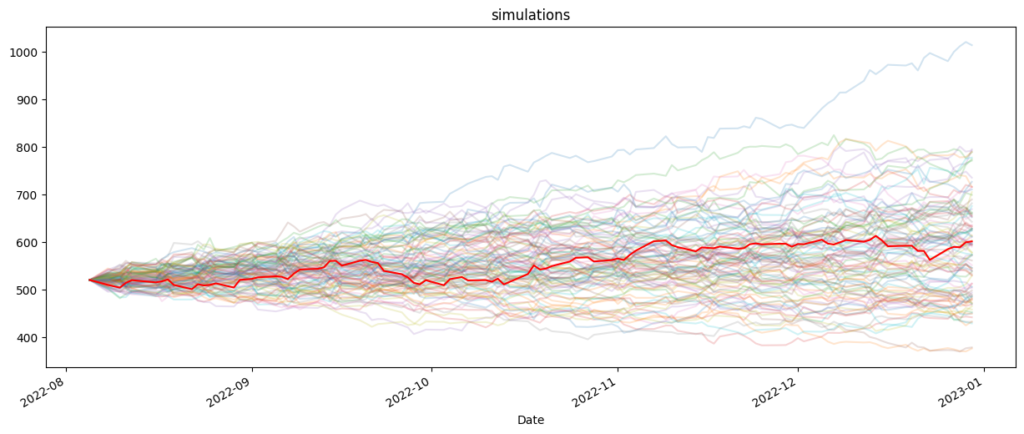
plot_title = 'GBM Simulations'
time_period = adjusted_close_prices[last_train_date:last_test_date].index
# Create a DataFrame for simulation results
gbm_simulations_df = pd.DataFrame(np.transpose(gbm_simulations), index=time_period)
# Plot the simulations and the actual data
simulations_plot = gbm_simulations_df.plot(alpha=0.2, legend=False, figsize=(15, 6))
actual_data_plot = adjusted_close_prices[last_train_date:last_test_date].plot(color='red')
plt.title(plot_title)
plt.show()
Variance Reduction Methods and Their Types
Variance reduction methods are techniques employed in statistics and simulation to reduce the variability or spread of data points around their expected value. They are especially valuable in Monte Carlo simulations and other statistical analyses, where high variance can lead to imprecise results. These methods aim to improve the accuracy and efficiency of estimates by minimizing the variance of the outcomes. Here, we’ll explore what variance reduction methods are and delve into different types.
What Are Variance Reduction Methods?
Variance reduction methods are strategies used to enhance the accuracy and efficiency of statistical estimates. They are particularly important in situations where random sampling is involved, such as Monte Carlo simulations. The primary objective of these methods is to reduce the spread of sample outcomes around the expected value, thereby enabling more precise estimates with a smaller number of samples.
Different Types of Variance Reduction Methods:
- Control Variates:
- Description: Control variates involve identifying a related random variable whose expected value is known. This variable is often chosen to be easy to compute.
- How It Works: By incorporating the control variate into the simulation, the variance of the estimate is reduced. The difference between the estimate and the control variate’s expected value is used to adjust the estimate.
- Applications: Commonly used in finance for option pricing and risk management. The Black-Scholes model is a classic example.
- Antithetic Variates:
- Description: Antithetic variates exploit the negative correlation between random variables.
- How It Works: Pairs of random variables with opposite signs are generated. When one variable is high, the other is likely to be low. This reduces variance.
- Applications: Commonly used in simulations to compare two similar scenarios with different input values, making it easier to identify sources of variance.
- Stratified Sampling:
- Description: Stratified sampling divides the sample space into strata (subgroups), each with its own sampling technique.
- How It Works: More samples are drawn from strata that are more critical, reducing variance by ensuring that important regions are well-represented.
- Applications: Useful when certain regions of the sample space are of particular interest, such as in reliability studies or risk assessments.
- Importance Sampling:
- Description: Importance sampling involves changing the probability measure under which a simulation is performed.
- How It Works: By using an alternative, often non-uniform, probability distribution, more samples are concentrated in regions of interest, reducing variance in the estimate.
- Applications: Widely used in various fields, including finance, physics, and engineering, to improve the efficiency and accuracy of simulations.
- Common Random Numbers:
- Description: Common random numbers involve using a shared source of randomness in two or more simulations.
- How It Works: Each sample in one simulation has a corresponding counterpart in the other, making it easier to identify sources of variance.
- Applications: Commonly used in optimization problems, finance, and reliability studies.
In summary, variance reduction methods are critical for improving the accuracy and efficiency of statistical estimates, especially in scenarios involving randomness. They encompass a range of techniques, each with its unique approach to reducing variance and enhancing the precision of results. The choice of method depends on the specific problem and the underlying data distribution.
Conclusion
Monte Carlo simulations, particularly when coupled with the Geometric Brownian Motion model, are invaluable tools for simulating stock price dynamics and understanding the probabilistic nature of financial markets. By embracing the power of randomness and iterative calculations, financial analysts and modelers gain valuable insights into pricing derivatives, managing risk, and making informed investment decisions. These simulations enable us to explore the many possible scenarios that financial markets may offer, making them a fundamental technique in modern finance.