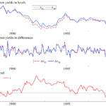
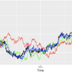
Cointegration is a critical concept in time series analysis, particularly in the field of econometrics and finance. It plays a fundamental role in understanding the long-term relationships between variables and has widespread applications in economics, finance, and other fields. In this article, we will explore the concept of cointegration, its mathematical derivation, and important concepts related to it. What is Cointegration? Cointegration is a statistical property of time series data that indicates a long-term, sustainable relationship between two or more variables. In simpler terms, it suggests that even though individual time series may be non-stationary (i.e., they exhibit trends or random variations), a linear combination of these variables can be stationary, which means it follows a stable pattern over time. The concept of cointegration is closely linked to the notion of stationarity. Stationarity implies that a time series has constant mean and variance over time. The derivation of cointegration involves a series of steps: Concepts Related to Cointegration Also read Optimizing Investment using Portfolio Analysis in R What is a Stationary and Non-Stationary Series? Stationary Series: A stationary time series is one where the statistical properties of the data do not change over time. In other words, it has a constant mean (average) and variance (spread) throughout its entire history. Additionally, the covariance between data points at different time intervals remains constant. Stationary series are often easier to work with in statistical analysis because their properties are consistent and predictable. Mathematically, a time series Y(t) is considered stationary if: Non-Stationary Series: A non-stationary time series, on the other hand, is one where the statistical properties change over time. This typically means that the series exhibits trends, seasonality, or other patterns that make its mean and/or variance variable across different time points. Non-stationary series can be more challenging to analyze and model because their behavior is not consistent. Non-stationary series often require transformations, such as differencing (taking the difference between consecutive data points), to make them stationary. Once made stationary, these differenced series can be easier to work with and can reveal underlying relationships that may not be apparent in the original non-stationary data. There are several statistical tests commonly used to check the stationarity of a time series. Here is a list of some popular stationarity tests, their mathematical formulations, and examples of their Python implementations using the statsmodels library: Augmented Dickey-Fuller (ADF) Test: The null hypothesis (H0) of the ADF test is that the time series has a unit root (i.e., it is non-stationary). The alternative hypothesis (H1) is that the time series is stationary. Kwiatkowski-Phillips-Schmidt-Shin (KPSS) Test: The KPSS test is used to test for the presence of a unit root (non-stationarity) around a deterministic trend. The null hypothesis (H0) is that the time series is stationary around a deterministic trend, while the alternative hypothesis (H1) is that it is non-stationary. Phillips-Perron (PP) Test: The PP test is similar to the ADF test and is used to test for the presence of a unit root. It has both a parametric and non-parametric version. Python Implementation: Elliott-Rothenberg-Stock (ERS) Test: The ERS test is another unit root test used to check for non-stationarity. The ERS test is not directly available in statsmodels, but you can find custom implementations or use alternative tests like ADF. Also Read Portfolio Optimization using Markowitz’s Mean Variance Method in R What is the Differencing method used for the stationary Series? Differencing involves taking the first difference of a time series to make it stationary. Differencing is a common method used to transform a non-stationary time series into a stationary one. Differencing Method: Differencing is relevant and significant in time series analysis for several reasons: 2. Mathematical Formulation: The differencing process involves subtracting each data point from the previous data point in the series. Here’s the mathematical formulation for differencing a time series Y(t): Differenced Series, Y'(t) = Y(t) – Y(t-1) In this equation: a valuable tool in time series analysis for making non-stationary data stationary, removing trends, and improving the reliability of statistical modeling and analysis. Its mathematical formulation is simple and involves subtracting each data point from the previous one, and the process is essential for preparing time series data for various analytical tasks. Which Co-Integration Tests can be used to test Time Series? Cointegration tests are used to determine whether two or more time series are cointegrated, meaning they have a long-term, stable relationship. Here is a list of popular cointegration tests, their explanations, mathematical formulations, and Python implementations using the statsmodels library: Engle-Granger Cointegration Test: The Engle-Granger test is a two-step procedure. In the first step, you regress one time series on the other(s) to estimate the cointegrating relationship. In the second step, you test the stationarity of the residuals from the regression. Johansen Cointegration Test: The Johansen test is a multivariate test used when dealing with more than two-time series. It helps determine the number of cointegrating relationships and the cointegration vectors. The Johansen test involves estimating a VAR (Vector Autoregressive) model and then testing the eigenvalues of a matrix to determine the number of cointegrating relationships. Phillips-Ouliaris Cointegration Test: The Phillips-Ouliaris test is a non-parametric cointegration test that doesn’t require the specification of a cointegrating vector. The test involves regressing the first-differenced time series on lagged levels and the first-differenced time series of the same variables. These cointegration tests are essential tools for determining the existence and nature of long-term relationships between time series data. The choice of which test to use depends on the number of time series involved and the assumptions of each test. A low p-value (typically less than 0.05) suggests the presence of cointegration, indicating a long-term relationship between the time series. What is a Cointegration Vector? A cointegration vector is a set of coefficients that defines the long-term relationship between two or more cointegrated time series. In a cointegration relationship, these coefficients specify how the individual time series move together in the long run, even though they may exhibit short-term fluctuations. Consider two-time series,

