Calculating Portfolio Beta and Portfolio Sensitivity to the Market using CAPM in R

The Capital Asset Pricing Model (CAPM) is a widely used financial framework for calculating the expected return on an investment based on its level of risk. Developed by William Sharpe, John Lintner, and Jan Mossin in the early 1960s, CAPM has become a fundamental tool in modern portfolio theory and investment analysis. It provides investors with a way to assess whether an investment offers an appropriate return relative to its risk and check for portfolio sensitivity with the market.

Also, read Optimizing Investment using Portfolio Analysis in R

To comprehend the derivation of the CAPM formula, it’s essential to understand its key components:

1. Risk-Free Rate (Rf): This represents the return on a risk-free investment, typically based on government bonds. It is the minimum return an investor expects to earn, as it carries no risk of loss.
2. Market Risk Premium (Rm – Rf): This measures the additional return expected from investing in the overall market (represented by a market index like the S&P 500) above the risk-free rate. It reflects the extra return required for taking on the inherent risk of the stock market.
3. Beta (β): Beta measures an asset’s sensitivity to market movements. A beta of 1 indicates that an asset moves in line with the market, while a beta greater than 1 suggests higher volatility than the market, and a beta less than 1 indicates lower volatility.

The Derivation of CAPM: The CAPM formula can be derived using principles from finance and statistics. It begins with the notion that the expected return on investment should compensate investors for both the time value of money (risk-free rate) and the risk associated with the investment.

The formula for CAPM is as follows:

Ri=Rf+βi(Rm−Rf)

Where:

• Ri is the expected return on the asset.
• Rf is the risk-free rate.
• βi is the beta of the asset.
• Rm is the expected return on the overall market.

Derivation Steps:

1. Expected Return vs. Risk: The expected return on an asset is the sum of the risk-free rate and a risk premium. This premium compensates investors for the risk they take by investing in a particular asset.
2. The Market Risk Premium: The risk premium can be calculated as the difference between the expected return on the market (Rm) and the risk-free rate (Rf), i.e., Rm−Rf.
3. The Role of Beta (β): Beta measures how much an asset’s returns are correlated with market returns. An asset with a beta of 1 will have returns that move in tandem with the market, while a beta less than 1 will be less volatile, and a beta greater than 1 will be more volatile.
4. Incorporating Beta into the Formula: To account for an asset’s risk relative to the market, the formula multiplies the market risk premium by the asset’s beta (βi). This scales the risk premium according to the asset’s sensitivity to market movements.
5. Final CAPM Formula: The derived formula, Ri=Rf+βi(Rm−Rf), combines the risk-free rate, market risk premium, and an asset’s beta to estimate the expected return on the asset.

CAPM (Capital Asset Pricing Model) is a widely used method for estimating the expected return on an investment based on its sensitivity to market movements. In this article, we will walk you through the step-by-step process of calculating the CAPM beta for a portfolio of stocks using R language. We will also discuss how sensitive your portfolio is to the market based on the calculated beta coefficient and visualize the relationship between your portfolio and the market using a scatterplot.

Step 1: Load Packages

Before we begin, make sure you have the necessary R packages installed. We’ll be using the tidyverse and tidyquant packages for data manipulation and visualization.

library(tidyverse)
library(tidyquant)

Step 2: Import Stock Prices

Choose the stocks you want to include in your portfolio and specify the date range for your analysis. In this example, we are using the symbols “SBI,” “ICICIBANK,” and “TATA MOTORS” with data from 2020-01-01 to 2023-08-01.

symbols <- c("SBIN.NS","ICICIBANK.NS","TATAMOTORS.NS")
prices <- tq_get(x  = symbols,
                 from="2020-01-01",
                 to="2023-08-01")

Step 3: Convert Prices to Returns (Monthly)

To calculate returns, we’ll convert the stock prices to monthly returns using the periodReturn function from the tidyquant package.

Asset_returns_tbl <- prices %>%
    group_by(symbol) %>%
    tq_transmute(select     = adjusted, 
                 mutate_fun = periodReturn,
                 period     = "monthly",
                 type       = "log") %>%
    slice(-1) %>%
    ungroup() %>%
    set_names(c("asset", "date", "returns"))

Step 4: Assign Weights to Each Asset

You can assign weights to each asset in your portfolio based on your preferences. Here, we are using weights of 0.45 for AMD, 0.35 for INTC, and 0.20 for NVDA.

symbols <- Asset_returns_tbl %>% distinct(asset) %>% pull()
weight <- c(0.25, 0.25, 0.50)
w_tbl <- tibble(symbols, weight)

Step 5: Build a Portfolio

Now, we’ll build a portfolio using the tq_portfolio function from tidyquant.

portfolio_returns_tbl <- Asset_returns_tbl %>%
    tq_portfolio(assets_col  = asset,
                 returns_col = returns,
                 weights = w_tbl, 
                 rebalance_on = "months",
                 col_rename = "returns")

Step 6: Calculate CAPM Beta

To calculate the CAPM beta, we need market returns data. In this example, we are using NASDAQ Composite (^IXIC) returns from 2020-01-01 to 2023-08-01.

market_returns_tbl <- tq_get(x    = "^IXIC",
                 from = "2012-12-31",
                 to   = "2017-12-31") %>%
    tq_transmute(select     = adjusted, 
                 mutate_fun = periodReturn,
                 period     = "monthly",
                 type       = "log",
                 col_rename = "returns") %>%
    slice(-1)

Portfolio_market_returns_tbl <- left_join(market_returns_tbl,
          portfolio_returns_tbl,
          "date") %>% 
    set_names("date", "market_returns", "portfolio_returns")

# Calculate CAPM beta
CAPM_beta <- Portfolio_market_returns_tbl %>%
    tq_performance(Ra = portfolio_returns,
                   Rb = market_returns,
                   performance_fun = CAPM.beta)

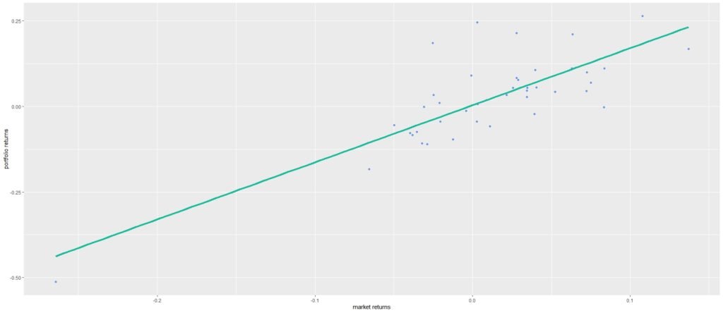
Step 7: Visualize the Relationship

Now, let’s create a scatterplot to visualize the relationship between your portfolio returns and market returns.

Portfolio_market_returns_tbl %>%
    ggplot(aes(x = market_returns, y = portfolio_returns)) +
    geom_point(color = "cornflowerblue") + 
    geom_smooth(method = "lm",
                se = FALSE,
                size = 1.5,
                color = tidyquant::palette_light()[3]) +
    labs(y = "Portfolio Returns",
         x = "Market Returns")

Portfolio Sensitivity to the Market

Based on the calculated CAPM beta of 1.67, your portfolio is generally more volatile than the market. A CAPM beta greater than 1 indicates a higher level of risk compared to the market. This observation is supported by the scatterplot, which shows a loose linear relationship between portfolio and market returns. While there is a trend, the data points do not strongly conform to the regression line, indicating greater volatility in your portfolio compared to the market.

For more such Projects in R, Follow us at Github/quantifiedtrader

Conclusion

The Capital Asset Pricing Model (CAPM) is a valuable tool for investors to determine whether an investment is adequately compensated for its level of risk. Its derivation highlights the importance of considering both the risk-free rate and an asset’s beta in estimating expected returns. CAPM provides a structured approach to making investment decisions by quantifying the relationship between risk and return in financial markets.

FAQs (Frequently Asked Questions):

Q1: What is CAPM, and why is it important for investors?

CAPM, or Capital Asset Pricing Model, is a financial model used to determine the expected return on an investment based on its risk and sensitivity to market movements. It’s important for investors because it helps assess the risk and return potential of an investment and make informed decisions.

Q2: How do I calculate CAPM beta for my portfolio?

To calculate CAPM beta, you need historical returns data for your portfolio and a market index, such as the S&P 500. Using regression analysis, you can determine the beta coefficient, which measures your portfolio’s sensitivity to market fluctuations.

Q3: What is the significance of a beta coefficient greater than 1?

A beta coefficient greater than 1 indicates that your portfolio is more volatile than the market. It suggests that your investments are likely to experience larger price swings in response to market movements, indicating a higher level of risk.

Q4: How can R language be used to calculate CAPM beta?

R language provides powerful tools for data analysis and regression modeling. By importing historical stock and market data, you can use R to perform the necessary calculations and determine your portfolio’s CAPM beta.

Q5: Why is it essential to understand portfolio sensitivity to the market?

Understanding portfolio sensitivity to the market is crucial for risk management. It helps investors assess how their investments might perform in different market conditions and make adjustments to their portfolios to achieve their financial goals while managing risk.