Are you looking to build your wealth and secure your financial future? Real estate investment could be the key to unlocking your financial success. In this comprehensive guide, we will delve into the world of real estate investment, exploring its core principles and concepts, and providing you with valuable insights to craft effective investment strategies. Understanding Real Estate Real estate is a tangible asset class consisting of properties, land, and resources. It plays a pivotal role in the global economy and is a cornerstone of wealth accumulation for many individuals and organizations. To navigate this intricate landscape, it’s crucial to grasp key concepts and principles. Core Principles and Concepts Building Investment Strategies Creating successful real estate investment strategies involves careful planning and consideration of your financial goals. Here’s a step-by-step approach: 1. Define Your Objectives: Clearly outline your investment goals, whether it’s income generation, long-term wealth, or a mix of both. 2. Budget and Financing: Determine your budget and explore financing options, including mortgage rates and terms. 3. Property Selection: Choose properties that align with your goals, budget, and risk tolerance. Analyze potential cash flow and appreciation. 4. Diversification: Spread your investments across different property types (e.g., residential, commercial) and geographic locations. 5. Risk Assessment: Evaluate and mitigate potential risks, including market fluctuations and unforeseen expenses. 6. Property Management: Decide whether to manage properties yourself or hire professionals. 7. Exit Strategy: Develop a plan for exiting investments to maximize returns. Concepts related to Real Estate investment Real estate investment offers a multitude of strategies, each tailored to different financial goals and risk tolerances. To make these strategies more accessible, they can be grouped into five categories: Business strategies, Starter strategies, Wealth building strategies, Debt strategies, and Passive strategies. Let’s delve into each category and explore these 15 strategies in detail. Business Strategies Starter Strategies Wealth Building Strategies Debt Strategies Passive Strategies Remember that these strategies are not mutually exclusive, and successful investors often combine them at different stages of their real estate journey. Conclusion Real estate investment is a dynamic and rewarding endeavor. By understanding the fundamental principles, concepts, and strategies, you can navigate this landscape with confidence. Remember that success in real estate investment requires a blend of knowledge, calculated risks, and a well-thought-out plan. Begin your journey towards financial prosperity today, and let real estate be your path to wealth accumulation. Frequently Asked Questions (FAQs) Q1: What is the best type of property to invest in? A1: The best type of property depends on your goals. Residential properties are great for rental income, while commercial properties can offer higher returns but come with more complexity. Q2: How can I finance my real estate investment? A2: Financing options include mortgages, loans, private money, and partnerships. The choice depends on your financial situation and investment strategy. Q3: Are there tax benefits to real estate investment? A3: Yes, real estate often offers tax advantages, such as deductions for mortgage interest, property taxes, and depreciation

Factor investing has gained tremendous popularity among investors seeking to enhance portfolio performance and manage risk. This investment approach involves targeting specific characteristics or factors that historically drive stock returns. By understanding and harnessing these factors, investors can potentially outperform the market over the long term. In this article, we’ll explore several powerful factor investing strategies and concepts that can help you achieve your financial goals. 1. Value Investing Value investing is one of the oldest and most well-known factor investing strategies. This approach focuses on identifying undervalued stocks trading below their intrinsic value. Investors look for companies with low price-to-earnings (P/E) ratios, low price-to-book (P/B) ratios, or high dividend yields. The underlying concept is that these undervalued stocks have the potential to appreciate as their true worth is recognized by the market. 2. Growth Investing In contrast to value investing, growth investing targets stocks with strong growth potential. Investors seek companies with high revenue and earnings growth rates. These stocks may have higher P/E ratios but are expected to deliver above-average returns due to their growth prospects. Growth investing is ideal for those willing to take on more risk in pursuit of substantial capital appreciation. 3. Dividend Yield Investing Dividend yield investing focuses on stocks that pay consistent and attractive dividends. The concept here is that companies with a history of dividend payments tend to be more stable and financially sound. By investing in dividend-paying stocks, investors can generate a steady income stream and benefit from potential capital appreciation. 4. Quality Investing Quality investing emphasizes the financial health and stability of a company. Investors look for stocks with strong balance sheets, low debt levels, and consistent profitability. Quality stocks are considered less risky and are often seen as defensive options during market downturns. 5. Momentum Investing Momentum investing capitalizes on the idea that stocks that have performed well in the recent past will continue to do so in the near future. Investors identify stocks with strong price momentum, believing they will gain further value. This strategy can be riskier as it relies on trends that may change quickly, but it can also yield significant returns. 6. Low Volatility Investing Low volatility investing focuses on stocks with historically lower price fluctuations. The concept is that these stocks offer more stability and reduced risk. While they may not experience rapid growth, they can provide steady returns and help protect portfolios during market volatility. 7. Size (Small-Cap and Large-Cap) Investing Size-based investing involves targeting stocks based on their market capitalization. Small-cap stocks, with smaller market capitalizations, often offer higher growth potential but come with increased risk. Large-cap stocks, on the other hand, are generally more stable but may have limited growth prospects. Investors can choose between these strategies based on their risk tolerance and return expectations. 8. Multifactor Investing Multifactor investing combines several of the above factors into a single strategy. By diversifying across factors like value, growth, and quality, investors aim to achieve a well-rounded portfolio that can perform in various market conditions. Multifactor investing seeks to balance risk and reward, providing a comprehensive approach to factor-based investing. 9. Earnings Yield Investing Earnings yield is the inverse of the P/E ratio. This strategy involves seeking stocks with high earnings yields, indicating that the company’s earnings are substantial relative to its market value. 9. Price-to-Sales (P/S) Ratio Investing The P/S ratio measures a company’s stock price relative to its revenue. Investors using this strategy look for stocks with low P/S ratios, indicating potential undervaluation. 10. Shareholder Yield Investing Shareholder yield combines dividends, stock buybacks, and debt reduction. This approach identifies stocks that return value to shareholders through various channels. 11. Equal Weight Investing In contrast to market capitalization-based weighting, equal weight investing assigns the same weight to each stock in a portfolio. This approach reduces the dominance of large-cap stocks and enhances diversification. 12. Profitability Investing Profitability investing focuses on companies with high returns on equity (ROE) and strong profit margins. These stocks tend to exhibit resilience during economic downturns. 13. Low Beta Investing Low-beta stocks have lower volatility compared to the overall market. Investors seeking stability may opt for this strategy to reduce portfolio risk. 14. High Dividend Growth Investing This strategy targets stocks with a history of consistently increasing dividend payouts. It combines income generation with the potential for capital appreciation. 15. Volatility Factor Investing Volatility factor investing capitalizes on the historical relationship between low volatility and strong returns. Stocks with lower price swings are considered safer investments. 16. Environmental, Social, and Governance (ESG) Investing ESG investing integrates environmental, social, and governance factors into investment decisions. It allows investors to align their portfolios with ethical and sustainable values. 17. Smart Beta Strategies Smart beta strategies combine factors like value, growth, and low volatility to create customized investment approaches. These strategies aim to outperform traditional market-cap-weighted indices Conclusion Factor investing opens the door to a world of possibilities for investors looking to enhance their portfolios. These strategies provide a structured approach to harnessing the power of specific stock characteristics. By understanding and implementing factor investing strategies, you can work toward your financial goals while managing risk effectively. Remember that a well-rounded investment approach may include multiple factors and ongoing research to adapt to changing market conditions. FAQs (Frequently Asked Questions) Q1: What is factor investing? Factor investing is an investment approach that targets specific characteristics, or factors, known to influence stock returns. These factors include value, growth, dividend yield, and more. Q2: How do factor investing strategies work? Factor investing strategies work by selecting stocks based on predefined factors like value, growth, or low volatility. Portfolios are constructed to emphasize these chosen factors. Q3: Are factor investing strategies suitable for all investors? Factor investing strategies can be tailored to suit different risk tolerances and objectives. However, it’s crucial to align the strategy with your financial goals. Q4: Can factor investing be combined with other investment approaches? Yes, factor investing can complement other strategies within a diversified portfolio. Combining factors can

Factor Analysis and Principal Component Analysis (PCA) are powerful statistical methods that help uncover hidden patterns and latent variables within data, making them valuable tools across a range of disciplines, including finance, psychology, and data analysis. Data is abundant in various forms, but its value lies in its structure, which transforms raw data into meaningful information. The curse of dimensionality arises when too many variables are involved, leading to sparse data and overfitting in predictive models. Dimensionality reduction techniques like PCA and Factor Analysis help overcome this challenge by creating composite dimensions to represent original features while reducing scatteredness in the data. In finance, these techniques take on a unique role in the form of factor investing. Factor investing involves identifying and leveraging key factors that contribute to asset returns. By understanding these underlying factors, investors aim to construct portfolios that outperform traditional market benchmarks. What is Principal Component Analysis (PCA)? What is Factor Analysis (FA)? Difference between Principal Component Analysis and Factor Analysis PCA aims to explain cumulative variance in variables.PCA components are derivedPCA explains all variancePCA calculates componentsPCA interprets weights as correlationsPCA uses correlations for eigenvectorsPCA specifies variables and estimates weights FA focuses on explaining covariances or correlations between variables.FA factors are latent elements.FA has an error term unique to each variableFA defines factors.FA as factor loadings.FA estimates optimal weights.FA specifies factors and estimates factor returns. Uses of PCAImage processing for facial recognition and computer vision.Investment analysis to predict stock returns.Genomic studies using gene expression measurements.Customer profiling in banking and marketing.Clinical studies in healthcare and food science.Analyzing psychological scales. Uses of Factor AnalysisDiversifying stock portfolios.Analyzing customer engagement in marketing.Improving employee effectiveness in HR.Customer segmentation in insurance or restaurants.Decision-making in schools and universities.Exploring socioeconomic status and dietary patterns.Understanding psychological scales. Use PCA when the goal is to reduce correlated predictors into independent components. Use FA when the aim is to understand and test for latent factors causing data variation. The idea behind using PCA to derive factors is purely mathematical/statistical in nature.  Whereas before, where we derived factors from observable economic phenomena, PCA attempts to capture underlying representations of the data that may not be able to hold a meaning that we can understand in nature. The goal of PCA is to reduce the dimensionality of data into “factors” that are powerful enough to “summarize” the population.  It is meant to convert a set of potentially correlated data into a set of linearly uncorrelated variables.  This process is able to both capture and diversify correlated data into separate values that have explanatory power. Factor investing, a strategy used in finance to enhance portfolio returns, can be significantly enriched by incorporating Principal Component Analysis (PCA). PCA is a statistical method that facilitates dimensionality reduction and data visualization. It transforms a dataset with multiple variables into a lower-dimensional representation, while retaining the essential information present in the original data. The application of PCA in factor investing involves several crucial steps: The application of PCA and factor analysis in finance can provide several advantages: In practice, factor analysis and PCA help investors uncover the latent factors that drive asset returns. These factors can include size, value, momentum, quality, and volatility, among others. The mathematical rigor of PCA ensures that these factors are extracted based on their ability to explain the variance in the asset returns. Once the factors are identified, investors assign weights to each factor based on their significance. Factors with higher eigenvalues, which explain more variance, receive higher weights in constructing portfolios. These weights dictate how much exposure the portfolio has to each factor. Factor investing using PCA is not a static process but an ongoing one. Portfolios must be monitored and rebalanced regularly to adapt to changing market dynamics. Furthermore, decisions about the number of factors to consider must be made thoughtfully, as this can significantly impact portfolio performance. Conclusion Factor investing using PCA and factor analysis is a sophisticated approach that leverages statistical techniques to uncover and harness the underlying factors driving asset returns. By doing so, investors aim to build portfolios that are more resilient, diversified, and capable of delivering superior risk-adjusted returns, making these techniques invaluable tools in the ever-evolving world of finance. Frequently Asked Questions (FAQs) 1. What is factor investing, and how does it relate to Principal Component Analysis (PCA)? Factor investing is a strategy in finance that focuses on specific attributes or factors that drive the performance of assets in a portfolio. PCA is a statistical technique used in factor investing to identify and quantify these factors by reducing the dimensionality of data and uncovering underlying patterns. 2. How does PCA help in factor investing? PCA helps factor investing by extracting the most important information from a high-dimensional dataset of asset returns. It identifies latent factors that influence asset performance, enabling investors to construct portfolios that capture these factors’ risk premia. 3. What are some common factors in factor investing? Common factors in factor investing include size, value, momentum, quality, and volatility. These factors have been extensively studied and are known to impact asset returns. 4. What is the importance of data standardization in PCA for factor investing? Data standardization is crucial in PCA to ensure that all variables are on the same scale. This prevents variables with larger magnitudes from dominating the analysis and ensures that factors are extracted based on their economic significance rather than their scale. 5. How are factor weights determined in factor investing with PCA? Factor weights are assigned based on the importance of the factors, as measured by their eigenvalues (explained variance). Factors with higher eigenvalues receive greater weights in constructing the portfolio. 6. Why is monitoring and rebalancing important in factor investing with PCA? Factor exposures can change over time due to market conditions. Regular monitoring and rebalancing of the portfolio are essential to maintain the desired factor allocations and ensure that the portfolio remains aligned with the chosen factors. 7. What are the benefits of incorporating PCA into factor investing strategies? Incorporating PCA into factor investing

In the world of finance, determining the value of a company’s stock is a crucial task for investors and analysts. To assist in this endeavor, a wide range of equity valuation models have been developed. In this comprehensive guide, we’ll delve into more than some of these models, each offering a unique perspective on how to assess the worth of a company’s equity. Dividend Discount Model (DDM) DDM values a stock by calculating the present value of expected future dividend payments. It assumes that a stock’s value is the sum of all anticipated dividend payments. The DDM, or Dividend Discount Model, is a financial valuation method used to estimate the intrinsic value of a stock by considering its expected future dividend payments. This model is based on the idea that the present value of all anticipated future dividends represents the fundamental value of a company’s equity. Here’s a more detailed explanation of the DDM: Components of the DDM: The Basic DDM Formula: The formula for the basic Dividend Discount Model can be expressed as follows: Two Common Variations of DDM: Gordon Growth Model (Constant Growth Model): This is a simplified version of DDM that assumes dividends will grow at a constant rate indefinitely. The formula for the Gordon Growth Model is Two-Stage DDM: Recognizing that many companies do not maintain a constant growth rate indefinitely, the Two-Stage DDM divides the valuation into two stages. In the first stage, dividends grow at one rate, and in the second stage, they grow at a different rate. This model is more suitable for companies with changing growth patterns. The DDM is one of the fundamental methods used in stock valuation. However, it has limitations. It assumes that dividends will be paid and that their growth will be constant or follow a predictable pattern. This makes it less applicable for companies that do not pay dividends or have erratic dividend policies. In such cases, alternative valuation methods like the Discounted Cash Flow (DCF) model may be more appropriate. Additionally, the DDM is sensitive to changes in the discount rate, making the choice of an appropriate rate crucial for accurate valuation. Discounted Cash Flow (DCF) DCF stands for Discounted Cash Flow, which is a financial valuation method used to estimate the intrinsic value of an investment, typically a company, by discounting its expected future cash flows to their present value. It’s based on the principle that the value of money today is worth more than the same amount in the future. The DCF model allows you to estimate the value of an investment based on the expected cash flows it will generate in the future while considering the time value of money. This method is widely used in finance and investment analysis to make decisions about whether an investment is undervalued or overvalued based on its estimated intrinsic value. Price-to-Earnings (P/E) Ratio Model The P/E ratio compares a stock’s current market price to its earnings per share (EPS). The intrinsic value is estimated by multiplying the expected EPS by a chosen P/E ratio. 6. Price-to-Book (P/B) Ratio Model: This model evaluates a stock’s value relative to its book value per share, which is the net asset value. 7. Price-to-Sales (P/S) Ratio Model: The P/S ratio compares a stock’s market price to its revenue per share. It’s particularly useful for companies with low or negative earnings. 8. Comparable Company Analysis (CCA): CCA compares a company’s valuation metrics (P/E, P/B, etc.) to those of industry peers to determine its relative value. 9. Precedent Transaction Analysis (PTA): PTA assesses a company’s value based on the prices paid for similar companies in past merger and acquisition transactions. 10. Earnings Multiplier Models (Growth and Value): These models assess a stock’s intrinsic value by applying a multiplier (e.g., P/E ratio) to the company’s expected earnings or earnings growth rate. 11. Residual Income Models: These models value a stock based on the economic profit it generates, which is the profit exceeding the cost of capital. 12. Asset-Based Models: Asset-based models calculate a stock’s value based on the fair market value of its tangible and intangible assets, minus liabilities. 14. Monte Carlo Simulation: It uses probabilistic models to estimate a range of possible valuations based on multiple assumptions and scenarios. 15. Comparable Transactions Analysis (CTA): CTA analyzes a company’s historical transactions to assess its current value. Graham’s Formula This formula values a stock based on a combination of earnings and bond yields. The Graham Formula, also known as the Benjamin Graham Formula or the Graham Intrinsic Value Formula, is a straightforward method used to estimate the intrinsic value of a stock. It was developed by Benjamin Graham, an influential value investor and the mentor of Warren Buffett. This formula is relatively simple and is based on the relationship between a stock’s earnings per share (EPS), its expected long-term growth rate, and the investor’s required rate of return. The Graham Formula can be expressed as follows: Graham Formula In this formula: The Graham Formula is a quick and simple tool for assessing the intrinsic value of a stock. However, it has limitations and assumptions: 17. Capital Asset Pricing Model (CAPM): CAPM uses expected return, the risk-free rate, and beta (a measure of a stock’s risk) to estimate a stock’s required rate of return. 18. Arbitrage Pricing Theory (APT): APT considers multiple factors impacting stock returns and uses them to estimate a stock’s expected return. 19. PEG Ratio: The PEG (Price/Earnings-to-Growth) ratio incorporates a company’s growth rate into the P/E ratio, offering a more comprehensive view of valuation. 20. Earnings Before Interest and Taxes (EBIT) Multiple: It compares a company’s value to its earnings before interest and taxes. 21. Earnings Before Interest, Taxes, Depreciation, and Amortization (EBITDA) Multiple: Similar to EBIT multiple, but includes depreciation and amortization expenses. 22. Liquidation Value: This model calculates equity value based on the liquidation of a company’s assets, often used in bankruptcy scenarios. 23. Sum-of-the-Parts Valuation: It values a company as the sum of the values of its

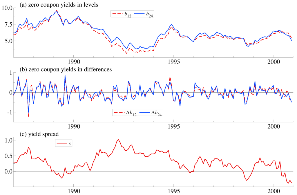
Fixed-income analysis is a crucial aspect of the investment world, playing a pivotal role in portfolios for both individuals and institutions. In this article, we will explore the key concepts of fixed-income analysis, the importance of bonds in a diversified portfolio, and how to conduct a comprehensive evaluation. Whether you’re a novice or an experienced investor, understanding fixed-income analysis is paramount for making informed financial decisions. What is Fixed-Income Analysis? Fixed-income analysis, also known as bond analysis, is the process of evaluating and assessing various aspects of fixed-income securities, primarily bonds. Fixed-income securities are debt instruments that pay investors periodic interest payments (known as coupons) and return the principal amount at maturity. These investments are considered less risky compared to equities, making them an attractive option for income generation and capital preservation. Why Invest in Bonds? Before delving into fixed-income analysis, let’s understand why bonds are a crucial component of investment portfolios: Key concepts Bonds: Debt securities that pay periodic interest and return the principal at maturity. They represent a form of debt or borrowing. They are essentially IOUs issued by various entities, such as governments, corporations, or municipalities, to raise capital. When you invest in a bond, you are lending money to the issuer in exchange for periodic interest payments, known as coupons, and the return of the principal amount at a specified maturity date. Yield: The income generated by a bond as a percentage of its face value. Yield refers to the return on an investment and is usually expressed as a percentage. It represents the income generated by an investment relative to its cost or current market value. Yield can take on various forms depending on the type of investment, but it generally indicates how much an investor can expect to earn from an investment over a specific period. Yield to Maturity (YTM): YTM represents the total return an investor can expect to receive if the bond is held until it matures. It considers not only the periodic interest payments (coupons) but also any capital gains or losses if the bond was purchased at a discount or premium to its face value. Coupon Rate: The coupon rate is the fixed periodic interest rate that the issuer of the bond agrees to pay to bondholders. It is expressed as a percentage of the bond’s face value or par value. The coupon rate determines the number of periodic interest payments that bondholders will receive throughout the life of the bond. Face Value (Par Value): The nominal value of a bond, which is returned to the investor at maturity. Maturity Date: The date when the principal amount of a bond is due to be repaid. Duration Duration is a financial metric used to measure the sensitivity of a bond’s price to changes in interest rates. It represents the weighted average time it takes to receive the bond’s cash flows, including coupon payments and the return of principal at maturity. Duration is typically expressed in years and helps investors assess and manage the interest rate risk associated with bonds. A higher duration implies greater price sensitivity to interest rate changes, while a lower duration suggests less sensitivity. Yield Curve The yield curve is a graphical representation of the interest rates (yields) on bonds with similar credit quality but different maturities at a specific point in time. It’s a critical tool in finance and economics because it provides insights into the expectations of future interest rates, economic conditions, and investor sentiment. Here’s an explanation of the yield curve and associated topics: 1. Yield Curve Shapes: 2. Term Structure of Interest Rates: 3. Factors Influencing the Yield Curve: 4. Uses of the Yield Curve: 5. Spot and Forward Rates: 6. Yield Spread: Inflation-Linked Bonds (TIPS): Bonds whose principal adjusts with inflation. Callable Bonds: Bonds that can be redeemed by the issuer before maturity. Puttable Bonds: Bonds that give the investor the right to sell them back to the issuer before maturity. Sovereign Bonds: Bonds issued by governments. Corporate Bonds: Bonds issued by corporations. Municipal Bonds (Munis): Bonds issued by state and local governments. Zero-Coupon Bonds: Bonds that don’t pay periodic interest but are sold at a discount to face value. Floating-Rate Bonds: Bonds with variable interest rates tied to a benchmark. Accrued Interest: The interest that has accumulated on a bond since its last coupon payment. Bond Ladder: A portfolio of bonds with staggered maturities. Credit Spread: The difference in yields between corporate bonds and government bonds. Nominal Yield: The coupon rate stated on a bond. Real Yield: The yield adjusted for inflation. Yield Curve Flattening: When the gap between short-term and long-term yields narrows. Yield Curve Steepening: When the gap between short-term and long-term yields widens. Treasury Bonds: Government bonds with maturities typically over 10 years. Treasury Notes: Government bonds with maturities typically between 2 and 10 years. Treasury Bills: Short-term government bonds with maturities of one year or less. Bond Fund: A mutual fund or exchange-traded fund (ETF) that invests in bonds. Yield to Call (YTC): The yield if a callable bond is called before maturity. Collateralized Debt Obligations (CDOs): Complex securities backed by pools of bonds. Securitization: The process of pooling and repackaging loans into securities. Callable/Convertible Preferred Stock: Preferred stock with features of both bonds and stocks. Laddered Bond Strategy: A strategy where bonds with different maturities are bought to spread risk. Term Structure of Interest Rates: The relationship between interest rates and time to maturity. Duration Matching: Aligning the duration of assets with liabilities to manage risk. Credit Default Swaps (CDS): Derivative contracts used to hedge against credit risk. Covenant: Legal clauses in bond agreements that specify issuer obligations and investor rights. Amortization: The gradual reduction of a bond’s principal through periodic payments. Yield to Worst (YTW): The lowest yield an investor can expect if a bond is called or matures early. Duration-Convexity Rule A guideline states that bond prices move inversely to changes in interest rates; duration predicts the direction, while convexity predicts the magnitude. The

In the world of finance, understanding the composition and style of investment portfolios is paramount. Style Analysis, a powerful tool, offers insights that go beyond traditional metrics. In this article, we’ll explore the concept of Style Analysis, its methodologies, applications, and how it provides investors with a deeper understanding of their portfolios. Understanding Style Analysis: Style Analysis is a quantitative technique used to dissect the underlying factors that contribute to the performance of an investment portfolio. It goes beyond asset allocation to reveal the portfolio’s style or investment characteristics. The Four Common Investment Styles: Methodologies of Style Analysis: Applications of Style Analysis: Benefits of Style Analysis: Conclusion: Style Analysis is a valuable tool in the toolkit of modern portfolio managers and investors. It empowers them to gain deeper insights into their investment style, make more informed decisions, and manage their portfolios effectively. In an increasingly complex investment landscape, Style Analysis provides the clarity needed to navigate the world of finance with confidence.

In the intricate world of finance, achieving the perfect balance between risk and reward is the Holy Grail for investors. Risk Parity Strategies, a dynamic approach to portfolio management, offer a solution. In this article, we’ll dive deep into the concept of Risk Parity, exploring its principles, applications, benefits, and how it’s reshaping the way investors approach asset allocation. Understanding Risk Parity: Risk Parity is a portfolio strategy designed to balance risk across asset classes, aiming to optimize returns while managing risk effectively. Traditional portfolios often allocate assets based on a fixed percentage (e.g., 60% stocks, 40% bonds). In contrast, Risk Parity focuses on equalizing risk contributions from each asset class. Principles of Risk Parity: Risk Parity Strategies: There are different approaches to implementing Risk Parity: Real-World Applications: Risk Parity Strategies have gained traction across various investment avenues: Benefits of Risk Parity: Conclusion: Risk Parity Strategies offer a compelling alternative to traditional portfolio allocation methods. By emphasizing risk diversification and volatility-based allocation, investors aim to achieve more balanced and potentially rewarding portfolios. As the financial landscape evolves, Risk Parity is redefining how investors approach asset allocation, offering a path to more robust and balanced investment portfolios.

In the ever-evolving landscape of finance, investors are constantly seeking ways to optimize returns while managing risk. Factor Investing, a strategy gaining immense popularity, offers a systematic approach to achieving these goals. This article dives deep into the world of Factor Investing, exploring its concepts, strategies, real-world applications, and the potential advantages it brings to the realm of investment. Understanding Factor Investing: Factor Investing, also known as Smart Beta or Style Investing, is based on the idea that specific factors or characteristics drive asset returns. These factors can include size, value, momentum, quality, and low volatility, among others. Instead of focusing solely on individual securities, Factor Investing emphasizes exposure to these factors to enhance portfolio performance. Key Factors in Factor Investing: Factor Investing Strategies: Factor Investing strategies can be broadly categorized into two types: Real-World Applications: Factor Investing has found extensive applications across the financial industry: Advantages of Factor Investing: Conclusion: Factor Investing represents a transformative approach to portfolio construction and risk management. By understanding and harnessing the power of systematic factors, investors can potentially achieve their financial objectives with greater efficiency and precision. As this approach continues to gain prominence, Factor Investing is poised to reshape the investment landscape, offering a new dimension of control and performance optimization for investors worldwide.

In the world of finance, understanding human behavior is as crucial as crunching numbers. Behavioral Finance, a branch of economics, explores how psychological biases and emotions influence financial decisions. This article delves into the intriguing realm of Behavioral Finance Theories, shedding light on the quirks of human decision-making that shape the financial landscape. Traditional Finance vs. Behavioral Finance: Traditional Finance theories have long assumed that investors are rational beings who make decisions solely based on objective information. However, Behavioral Finance challenges this notion. It acknowledges that human emotions, cognitive biases, and heuristics often lead to irrational decisions, deviating from traditional models. Key Behavioral Finance Theories: Practical Implications Behavioral Finance Theories have profound implications for investors and financial professionals: Conclusion Behavioral Finance Theories have transformed our understanding of financial decision-making. By acknowledging the influence of emotions and cognitive biases, these theories offer a more nuanced perspective on how markets operate and why investors behave the way they do. In the complex world of finance, appreciating the human element is as vital as crunching the numbers. As we continue to unravel the mysteries of Behavioral Finance, we gain valuable insights into the intricate dance between human psychology and financial markets.

In the dynamic realm of finance, precision is key. Investors are constantly seeking sophisticated tools to navigate markets and optimize their portfolios. Multi-Factor Models have emerged as a game-changer in asset pricing and investment strategy. In this insightful article, we’ll delve into the world of Multi-Factor Models, exploring their concepts, applications, and how they revolutionize the understanding of asset pricing. Understanding Multi-Factor Models: Multi-factor models extend beyond the traditional one-factor models like the Capital Asset Pricing Model (CAPM). They acknowledge that asset returns are influenced by multiple factors, not just market risk. These factors can include size, value, momentum, volatility, and more. By considering a broader spectrum of influences, Multi-Factor Models provide a more comprehensive view of asset pricing. This general formula demonstrates how a Multi-Factor Model combines multiple factors, each with its respective beta coefficient, to estimate the expected return of an asset. The model aims to capture the influence of various factors on asset returns, providing a more comprehensive view of pricing and risk assessment. Applications: Multi-factor models have far-reaching applications in finance: The Power of Multi-Factor Models: Multi-factor models offer several advantages: Challenges and Considerations: While Multi-Factor Models provide valuable insights, they are not without challenges: Conclusion Multi-factor models represent a significant advancement in asset pricing and investment strategy. They recognize the multifaceted nature of asset returns and empower investors to make more informed decisions. By understanding and utilizing these models, investors can enhance their portfolio construction, risk management, and asset valuation processes. In an ever-evolving financial landscape, Multi-Factor Models provide a powerful tool for unlocking investment opportunities and achieving financial goals.

In the complex landscape of financial markets, investors seek tools that can help them make more informed decisions. One such tool that has transformed the way we analyze and understand asset returns is the Fama-French Three-Factor Model. Developed by renowned economists Eugene Fama and Kenneth French, this model offers a sophisticated approach to asset pricing and portfolio management. In this comprehensive article, we will delve into the Fama-French Three-Factor Model, exploring its concepts, mathematical framework, practical applications, and how it has reshaped the world of finance. Understanding the Fama-French Three-Factor Model: The Fama-French Three-Factor Model builds on the Capital Asset Pricing Model (CAPM) by incorporating additional factors that affect asset returns. Unlike CAPM, which considers only market risk, this model recognizes that other factors like size and value can significantly impact an asset’s performance. Mathematical Framework: At the core of the Fama-French Model are three factors that capture different sources of risk: The mathematical formula for the Fama-French Three-Factor Model is as follows: Here’s a breakdown of the components: Real-World Applications The Fama-French Three-Factor Model has profound implications in various financial areas: Enhancing Investment Strategy The Fama-French Three-Factor Model offers several advantages: Conclusion The Fama-French Three-Factor Model has revolutionized the field of finance by recognizing that asset returns are influenced by more than just market risk. By understanding its concepts and mathematical framework, investors and analysts can make more informed investment decisions, construct well-diversified portfolios, and manage risks effectively. Incorporating this model into your investment strategy can provide a valuable edge in today’s dynamic financial landscape.

In the world of finance, making informed investment decisions is the key to success. The Black-Litterman Model, developed by Fischer Black and Robert Litterman, offers a sophisticated approach to asset allocation and portfolio optimization. In this article, we will delve into the Black-Litterman Model, exploring its concepts, mathematical framework, real-world applications, and how it can enhance your investment strategy. Understanding the Black-Litterman Model: Concepts: The Black-Litterman Model is a groundbreaking tool used in modern portfolio management. It addresses the limitations of traditional Mean-Variance Optimization by incorporating the subjective views of investors into the asset allocation process. Mathematical Framework: The heart of the Black-Litterman Model lies in its mathematical formulation, which can be represented as follows: Here’s a breakdown of the components: The Black-Litterman Model combines historical data, market views, and investor views to estimate expected returns. It provides a more realistic approach to asset allocation, especially when historical data might not accurately reflect current market conditions. Real-World Applications The Black-Litterman Model is widely applied in various financial scenarios: Enhancing Investment Strategy The Black-Litterman Model offers several advantages: Conclusion: The Black-Litterman Model is a powerful tool that bridges the gap between quantitative analysis and subjective views in finance. By understanding its concepts and mathematical framework, investors and analysts can make more informed investment decisions, construct diversified portfolios, and manage risks effectively. Incorporating this model into your investment strategy can provide a valuable edge in today’s dynamic financial landscape.

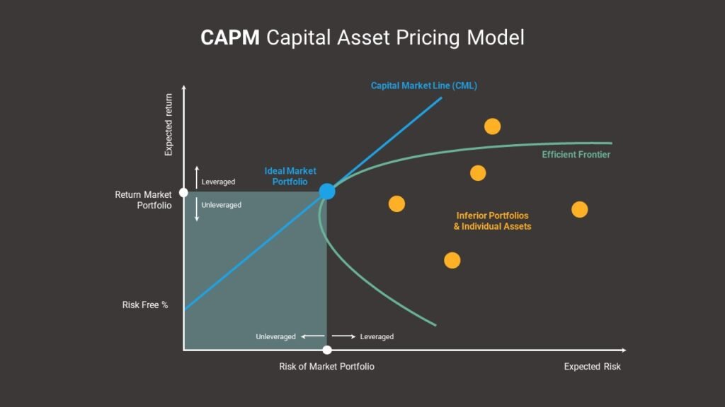
In the world of finance, achieving the right balance between risk and return is crucial for investors. One tool that has stood the test of time in helping investors make informed decisions is the Capital Asset Pricing Model (CAPM). Developed by financial scholars in the 1960s, CAPM offers valuable insights into asset pricing, portfolio construction, and risk management. In this article, we’ll provide a comprehensive understanding of the CAPM model, its historical background, how to apply it, its modern-day relevance, its drawbacks, and alternative theories. We’ll also explain the steps to implement CAPM effectively. Historical Background The story of CAPM began in the 1960s when financial theorists William Sharpe, John Lintner, and Jan Mossin introduced this groundbreaking framework. They sought to answer a fundamental question: How can investors optimize their portfolios to achieve the highest returns possible given a specific level of risk? Key Concepts At the heart of CAPM lie a few essential concepts: Mathematical Formulation The CAPM formula is expressed as follows: How to Apply CAPM Drawbacks and Criticisms While CAPM is influential, it’s not without its criticisms: How to Implement CAPM Implementing CAPM involves: Conclusion The Capital Asset Pricing Model (CAPM) is a valuable tool for investors seeking to understand the relationship between risk and return. While it has its critics, CAPM remains a foundational framework in finance, offering insights for investment decisions, portfolio management, and risk assessment. By applying CAPM alongside other models and factors, investors can achieve a more comprehensive understanding of financial markets.

Welcome to WordPress. This is your first post. Edit or delete it, then start writing!

Value at Risk, often abbreviated as VaR, is a vital concept in risk management, financial modeling, and decision-making. It provides a statistical measure of the potential loss an investment or portfolio might experience over a specified time horizon, at a given confidence level. This article provides an in-depth exploration of VaR, including its history, mathematical formulas, types, meanings, and how to interpret its significance. History of Value at Risk The concept of VaR traces its roots to the financial industry’s increasing need for risk assessment and management. It gained prominence in the late 20th century as a result of the following developments: The Mathematical Foundation of Value at Risk (VaR) At the core of VaR is a probability-based approach, often relying on statistical and mathematical models. Several formulas are used to calculate VaR, each tailored to different applications. Here, we present some of the most fundamental ones in LaTeX code: Where: This approach involves generating thousands of scenarios, simulating portfolio returns, and finding the xth percentile of the resulting distribution. Types of Value at Risk (VaR) Additional concepts related to Value at Risk (VaR) Parametric VaR for a Portfolio: For a portfolio of assets, the Parametric VaR is calculated by considering the portfolio’s weighted sum of asset returns. If Ri​ represents the return of asset i in the portfolio with weight wi​, the formula is:​ σp​ is the portfolio standard deviation. Cornish-Fisher VaR: This formula adjusts Parametric VaR to account for skewness and kurtosis in return distributions. It provides a more accurate estimate when returns are not normally distributed. S is the skewness of returns. K is the kurtosis of returns. Delta-Normal VaR: Delta-Normal VaR is used in options trading to calculate the change in the value of an option or derivative due to small changes in the underlying asset price ΔS is the change in the asset price. N−1(α) is the quantile of the standard normal distribution corresponding to the desired confidence level. Understanding the Meaning of Value at Risk (VaR) VaR quantifies the risk of a portfolio or investment, but understanding its significance is critical. Consider the following key points: Conclusion Value at Risk is a powerful tool for risk assessment and management. Its mathematical foundation, types, and interpretations offer a multifaceted perspective on potential losses. While it has become a standard in finance, it’s essential to grasp its assumptions and limitations to make informed decisions and safeguard portfolios against unforeseen risks.

Econometrics plays a pivotal role in the realm of economics by equipping researchers with essential tools for modeling based on empirical data. Among these tools, the technique of regression analysis stands out as a fundamental and versatile method. It serves as the cornerstone for understanding relationships, making predictions, and deriving valuable insights from economic data. Linear vs. Non-Linear Regression Analysis Regression models can be broadly classified into two categories: linear and non-linear. Linear regression analysis and non-linear regression analysis are the primary subfields within this domain. In this discussion, we will primarily focus on the intricacies of linear regression analysis. Linear regression analysis is a powerful statistical method employed in econometrics to establish relationships between variables in a linear fashion. Its primary objective is to fit a linear regression model to a given dataset, enabling economists and researchers to gain a deeper understanding of the underlying dynamics. What is Simple Linear Regression? Simple linear regression is a statistical method used to model the relationship between two variables: one independent variable (predictor) and one dependent variable (response). It’s a straightforward approach to understanding how changes in the independent variable influence the dependent variable. Think of it as a way to draw a straight line through data points, making predictions based on this linear relationship. At the heart of linear regression lies a fundamental distinction between two key variable types: the dependent variable (often referred to as the study variable), denoted as ‘y,’ and independent variables (also known as explanatory variables), denoted as ‘X,’ ‘X1,’ ‘X2,’ and so forth. The dependent variable ‘y’ is the focal point of our analysis, representing the outcome we aim to elucidate or predict. In contrast, independent variables ‘X’ encapsulate various factors that hold the potential to influence ‘y.’ Key Components Simple linear regression involves the following key components: Linearity vs. Non-Linearity: The core of understanding linearity in regression analysis lies in assessing the relationship between ‘y’ and the model parameters (‘β_0,’ ‘β_1,’ ‘β_2,’ …, ‘β_k’). Specifically, a model is deemed linear if all partial derivatives of ‘y’ with respect to each parameter remain independent of those parameters. Conversely, if any derivative depends on the parameters, the model is classified as non-linear. It’s vital to note that this classification pertains to the parameters themselves, not the independent variables. Linear Regression Equation with Interaction Terms: We can extend the linear regression equation to include interaction terms. Interaction terms capture the joint influence of two or more independent variables on the dependent variable. The equation takes this form: Here, the ‘β_3’ term quantifies how the interaction between ‘X_1’ and ‘X_2’ contributes to changes in ‘y.’ Multiple Linear Regression: The multiple linear regression equation accommodates multiple independent variables simultaneously. It expands the equation to encompass ‘p’ independent variables: The coefficients ‘β_1’ through ‘β_p’ measure the impact of each respective independent variable ‘X_1’ through ‘X_p’ on the dependent variable ‘y.’ Polynomial Regression: In situations where the relationship between ‘y’ and ‘X’ is nonlinear, polynomial regression steps in. It introduces higher-order terms of the independent variables to capture nonlinear patterns. The equation can extend to include quadratic terms: Here, ‘X_1^2’ represents the squared term of ‘X_1,’ allowing the model to capture curvature in the relationship. Use Cases and Applications Simple linear regression finds applications in various fields, including: The Process of Simple Linear Regression We’ll now break down the essential concepts of linear regression and dive deep into each step of the process. Step 1: Define the Problem The first thing we need to do is clearly state the problem we want to solve. What are we trying to find out, and what do we want to achieve with our analysis? Defining the problem sets the stage for everything that follows. Step 2: Choose the Right Variables Next, we need to pick the right things to study. These are called variables. Some variables are the ones we want to understand better (we call this the dependent variable), and others are factors that might affect our main variable (we call these independent variables). Step 3: Collect Good Data Having good information is crucial. We need to gather data on our chosen variables accurately. The data should be relevant and reliable, meaning it should give us a true picture of what we’re studying. Step 4: Create the Model Now, we come to the heart of linear regression: creating a model. A model is like a math equation that tells us how our dependent variable is connected to our independent variables. In a simple form, it looks like this: Step 5: Figure Out the Numbers To get our model ready, we need to figure out the values of β₀ and β₁. This is where math comes in. There are different methods for finding these numbers, such as the least-squares method, which aims to make our model as accurate as possible. Step 6: Fit the Model Once we have our numbers, we put them into our model equation. This is like fitting a puzzle piece into its place. The model is now ready to help us understand the relationship between our variables. Step 7: Check the Model We need to make sure our model is doing a good job. To do this, we check if it follows certain rules and assumptions. If it doesn’t, we might need to make some adjustments or consider a different approach. Step 8: Use the Model Finally, we can use our model to make predictions or draw conclusions. For example, if we were studying how the amount of sunlight affects plant growth, our model could help us predict how tall a plant might grow based on how much sunlight it gets. Objectives of Regression Analysis Regression analysis serves several pivotal objectives: – Relationship Exploration: It uncovers and quantifies relationships between the dependent variable ‘y’ and the independent variable ‘X.’ This exploration empowers researchers to gain valuable insights into the influencing factors. – Prediction: Fitted regression models enable accurate prediction. Once the parameters are estimated, you can forecast ‘y’ values for