quantedx.com

Understanding Greeks in Options Trading

In the realm of options trading, understanding the concept of moneyness and the intricate world of Greek letters is crucial. In this comprehensive guide, we will demystify these concepts while providing mathematical expressions for each term and delving into the intricacies of second-order Greeks. Moneyness: ATM, OTM, and ITM ATM (At The Money): ATM options occur when the strike price ($K$) closely matches the current stock price ($S$). Mathematically, it can be expressed as: K≈S For instance, a $50 strike call option would be ATM if the stock is trading at $50. OTM (Out of the Money): OTM options are those where exercising the option would not be advantageous at expiration. If an option has a strike price higher than the current stock price, we can express it as: K>S For instance, having a $40 call option when the stock is trading at $35 is an OTM scenario. ITM (In the Money): ITM options are favorable for exercising at expiration. When the strike price is lower than the current stock price, we can express it as: K<S For instance, a $40 call option is ITM when the underlying stock is trading above $40. Intrinsic and Extrinsic Value Options pricing comprises two fundamental components: intrinsic value (IV) and extrinsic value (EV). Intrinsic Value (IV): IV represents how deep an option is in the money. For call options, it is expressed as: Call​=max(S−K,0) For put options, it is calculated as: Put​=max(K−S,0) Extrinsic Value (EV): EV is often referred to as the “risk premium” of the option. It is the difference between the option’s total price and its intrinsic value: EV=Option Price−IV The Greeks: Delta, Gamma, Theta, Vega, and Rho Delta Delta measures how an option’s price changes concerning the underlying stock price movement. It can be expressed as: Δ=∂V/∂S​ Where: For stocks, Delta is straightforward, remaining at 1 unless you exit the position. However, with options, Delta varies, depending on the strike price and time to expiration. Gamma Gamma indicates how delta ($\Delta$) changes concerning shifts in the underlying stock’s price. Mathematically, it can be expressed as: Γ=∂Δ​/∂S Where: Gamma is the first derivative of delta and the second derivative of the option’s price concerning stock price changes. It plays a significant role in managing the dynamic nature of options. Theta Theta quantifies the rate of time decay in options, indicating how much the option price diminishes as time passes. It is mathematically expressed as: Θ=∂V/∂t​ Where: For long options, Theta is always negative, signifying a decrease in option value as time progresses. Conversely, short options possess a positive Theta, indicating an increase in option value as time elapses. Vega Vega gauges an option’s sensitivity to changes in implied volatility. The mathematical expression for vega is: ν=∂V/∂σ​ Where: High vega implies that option prices are highly sensitive to changes in implied volatility. Rho Rho evaluates the change in option price concerning variations in the risk-free interest rate. Its mathematical expression is: ρ=∂V/∂r​ Where: Rho’s impact on option pricing is generally less prominent than other Greeks but should not be overlooked. Utilizing Second-Order Greeks in Options Trading Second-order Greeks provide traders with a deeper understanding of how options behave in response to various factors. They offer insights into the more intricate aspects of options pricing and risk management. Let’s explore these second-order Greeks in greater detail and understand their significance. Vanna Vanna measures how the delta of an option changes concerning shifts in both the underlying stock price (S) and implied volatility. It combines aspects of both Delta and Vega. Mathematically, Vanna can be expressed as: νΔ​=∂Δ​/∂S∂σ Understanding Vanna is particularly valuable for traders who wish to assess how changes in both stock price and volatility can impact their options positions. It allows for more precise risk management and decision-making when these two critical variables fluctuate. Charm Charm quantifies the rate at which delta changes concerning the passage of time t. It evaluates how an option’s sensitivity to time decay varies as the option approaches its expiration date. Mathematically, Charm can be expressed as: ΘΔ=∂Δ​/∂t Charm is particularly valuable for traders employing strategies that rely on the effects of time decay. It helps in optimizing the timing of entry and exit points, enhancing the precision of options trading decisions. Vomma Vomma, also known as the volatility gamma, assesses how gamma changes concerning shifts in implied volatility. It is essentially the second derivative of gamma concerning volatility. Mathematically, Vomma can be expressed as: νΓ=∂Γ​/∂σ Vomma is essential for traders who want to understand the impact of changes in implied volatility on their options positions. It aids in adapting strategies to volatile market conditions, allowing traders to take advantage of changing market dynamics The behavior of the Greeks varies for different options trading strategies. Each strategy has its own objectives and risk profiles, which are influenced by the Greeks in unique ways. Let’s explore how the primary Greek variables – Delta, Gamma, Theta, Vega, and Rho – behave for some common options trading strategies: What are the differences between the Option Buyer and Option Seller strategies in terms of Option Greeks? Option buyers and option sellers, also known as writers, have fundamentally different approaches to options trading, and this is reflected in how the Greeks impact their strategies. Let’s explore the key differences between the two in terms of the Greeks: Managing Delta and Gamma for option sellers is crucial to control risk and optimize profitability. Here’s how option sellers can manage Delta and Gamma, along with the corresponding equations: Strategy involves a careful analysis of the components of the strategy. A Delta-neutral position means that the strategy’s sensitivity to changes in the underlying asset’s price is effectively balanced, resulting in a Delta of zero. Here’s how you can know that Delta is zero for a strategy: Can I make a long gamma and long theta strategy? It is challenging to create a strategy that is both “long gamma” and “long theta” simultaneously because these two Greeks typically have opposite characteristics. However, you can design

Understanding Greeks in Options Trading Read More »
Stylized Facts of Assets: A Comprehensive Analysis

In the intricate world of finance, a profound understanding of asset behavior is crucial for investors, traders, and economists. Financial assets, ranging from stocks and bonds to commodities, demonstrate unique patterns and characteristics often referred to as “stylized facts.” These stylized facts offer invaluable insights into the intricate nature of asset dynamics and play an instrumental role in guiding investment decisions. In this article, we will delve into these key stylized facts, reinforced by mathematical equations, to unveil the fascinating universe of financial markets in greater detail. Returns Distribution The distribution of asset returns serves as the foundation for comprehending the dynamics of financial markets. Contrary to the expectations set by classical finance theory, empirical observations frequently reveal that asset returns do not adhere to a normal distribution. Instead, they often exhibit fat-tailed distributions, signifying that extreme events occur more frequently than predicted. To model these non-normal distributions, the Student’s t-distribution is frequently employed, introducing the degrees of freedom (ν) parameter: Volatility Clustering Volatility clustering is a phenomenon where periods of heightened volatility tend to cluster together, followed by periods of relative calm. This pattern is accurately captured by the Autoregressive Conditional Heteroskedasticity (ARCH) model, pioneered by Robert Engle: Here, Leverage Effect The leverage effect portrays a negative correlation between asset returns and changes in volatility. When asset prices decline, volatility tends to rise. This phenomenon is aptly described by the GARCH (Generalized Autoregressive Conditional Heteroskedasticity) model: In this context, γ embodies the leverage effect. Serial Correlation Serial correlation, or autocorrelation, is the tendency of an asset’s returns to exhibit persistence over time. Serial correlation can be measured through the autocorrelation function (ACF) or the Ljung-Box Q-statistic: Here, Tail Dependence Tail dependence quantifies the likelihood of extreme events occurring simultaneously. This concept is of paramount importance in portfolio risk management. Copula functions, such as the Clayton or Gumbel copulas, are utilized to estimate the tail dependence coefficient (TDC): For the Clayton copula: For the Gumbel copula: Mean Reversion Mean reversion is the tendency of asset prices to revert to a long-term average or equilibrium level over time. This phenomenon suggests that when an asset’s price deviates significantly from its historical average, it is likely to move back toward that average. The Ornstein-Uhlenbeck process is a mathematical model that describes mean reversion: Where: Volatility Smile and Skew The volatility smile and skew refer to the implied volatility of options across different strike prices. In practice, options markets often exhibit a smile or skew in implied volatility. This means that options with different strike prices have different implied volatilities. The Black-Scholes model, when extended to handle such scenarios, introduces the concept of volatility smile, and skew. Long Memory Long memory, also known as long-range dependence, describes the persistence of past price changes in asset returns. This suggests that asset returns exhibit memory of past price movements over extended time horizons. The Hurst exponent (H) is often used to measure long memory in asset returns, with 0.5<H<1 indicating a positive long memory. Jumps and Leptokurtosis Asset returns frequently exhibit jumps or sudden large price movements. These jumps can lead to leptokurtic distributions, where the tails of the return distribution are thicker than a normal distribution. The Merton Jump-Diffusion model is used to capture this behavior, adding jumps to the standard geometric Brownian motion model: Where:

Stylized Facts of Assets: A Comprehensive Analysis Read More »

State-Space Models and Kalman Filtering: Unveiling the Hidden Dynamics

State-space models, often paired with Kalman filtering, are powerful tools for modeling and analyzing dynamic systems in various fields, including engineering, finance, economics, and more. These models excel in capturing hidden states and noisy observations, making them indispensable in predicting future states and estimating unobservable variables. In this detailed article, we will delve into the concepts of state-space models and Kalman filtering, providing the necessary equations and explaining their applications across different domains. Understanding State-Space Models A state-space model represents a system’s evolution over time as a pair of equations: the state equation and the observation equation. State Equation: xt​ is the state vector at time t, F is the state transition matrix, B is the control input matrix. , ut​ is the control input, wt​ is the process noise. Observation Equation: yt​ is the observation vector at time t. H is the observation matrix. vt​ is the observation noise. Applications: State-space models find applications in diverse fields: Kalman Filtering: The Hidden Inference Kalman Filter Equations: The Kalman filter combines noisy observations with a system’s dynamics to estimate the hidden state. It operates recursively, updating the state estimate as new observations arrive. Prediction Step: Predicted State: Predicted Error Covariance: Correction Step: Kalman Gain: Corrected State Estimate: Corrected Error Covariance:​ Applications: Kalman filtering is widely used in various fields: Extended Kalman Filter (EKF) In many real-world applications, the underlying dynamics are non-linear. The Extended Kalman Filter (EKF) extends the Kalman filter to handle non-linear state-space models. EKF Equations: The EKF introduces the concept of linearization to handle non-linear models. Prediction Step (Non-Linear): Predicted State: Predicted Jacobian Matrix: ​ Predicted Error Covariance: ​ Correction Step (Non-Linear): Kalman Gain: Corrected State Estimate: Corrected Jacobian Matrix: ​ Corrected Error Covariance: Applications: The EKF is applied in fields with non-linear models: Unscented Kalman Filter (UKF) The Unscented Kalman Filter (UKF) is an alternative to EKF for non-linear systems. It avoids linearization by approximating the mean and covariance of predicted and corrected states using a set of carefully chosen sigma points. UKF Equations: UKF equations replace the linearization step in the EKF with sigma points and their propagated estimates. Applications: UKF is employed in various non-linear applications: Conclusion State-space models and Kalman filtering, along with their extensions like EKF and UKF, are versatile tools for modeling dynamic systems and estimating hidden states. These techniques have widespread applications in fields ranging from economics to robotics, offering insights into complex, evolving processes. As computational power continues to grow, the utility of these models in uncovering hidden dynamics and making accurate predictions is poised to expand even further.

State-Space Models and Kalman Filtering: Unveiling the Hidden Dynamics Read More »

Markov Chain Monte Carlo (MCMC) Methods in Econometrics

Markov Chain Monte Carlo (MCMC) methods have revolutionized econometrics by providing a powerful toolset for estimating complex models, evaluating uncertainties, and making robust inferences. This article explores MCMC methods in econometrics, explaining the fundamental concepts, applications, and mathematical underpinnings that have made MCMC an indispensable tool for economists and researchers. Understanding MCMC Methods What is MCMC? MCMC is a statistical technique that employs Markov chains to draw samples from a complex and often high-dimensional posterior distribution. These samples enable the estimation of model parameters and the exploration of uncertainty in a Bayesian framework. Bayesian Inference and MCMC At the core of MCMC lies Bayesian inference, a statistical approach that combines prior beliefs (prior distribution) and observed data (likelihood) to update our knowledge about model parameters (posterior distribution). MCMC provides a practical way to sample from this posterior distribution. Markov Chains Markov chains are mathematical systems that model sequences of events, where the probability of transitioning from one state to another depends only on the current state. In MCMC, Markov chains are used to sample from the posterior distribution, ensuring that each sample is dependent only on the previous one. Key Concepts in MCMC Methods Metropolis-Hastings Algorithm The Metropolis-Hastings algorithm is one of the foundational MCMC methods. It generates a sequence of samples that converge to the target posterior distribution. Steps of the Metropolis-Hastings Algorithm: Gibbs Sampling Gibbs sampling is a special case of MCMC used when sampling from multivariate distributions. It iteratively samples each parameter from its conditional distribution while keeping the others fixed. Mathematical Notation (Gibbs Sampling): For parameters θ1​,θ2​,…,θk​: P(θi​∣θ1​,θ2​,…,θi−1​,θi+1​,…,θk​,X) Burn-In and Thinning MCMC chains often require a burn-in period where initial samples are discarded to ensure convergence. Thinning is an optional step that reduces autocorrelation by retaining only every �n-th sample. Mathematical Notation (Thinning): Thinned Samples: θ1​,θn+1​,θ2n+1​,… Applications in Econometrics MCMC methods find applications in various areas of econometrics: Bayesian Regression Models MCMC enables the estimation of Bayesian regression models, such as Bayesian linear regression and Bayesian panel data models. These models incorporate prior information, making them valuable in empirical studies. Mathematical Equation (Bayesian Linear Regression): Time Series Analysis Econometric time series models, including state space models and autoregressive integrated moving average (ARIMA) models, often employ MCMC for parameter estimation and forecasting. Mathematical Equation (State Space Model): Structural Break Detection MCMC methods are used to detect structural breaks in time series data, helping economists identify changes in economic regimes. Mathematical Equation (Structural Break Model): Challenges and Advances While MCMC methods have revolutionized econometrics, they come with computational challenges, such as long runtimes for large datasets and complex models. Recent advances in MCMC include: Conclusion MCMC methods have significantly enriched the toolkit of econometricians, allowing them to estimate complex models, make informed inferences, and handle challenging datasets. By embracing Bayesian principles and Markov chains, researchers in econometrics continue to push the boundaries of what can be achieved in understanding economic phenomena and making robust predictions. As computational resources continue to advance, MCMC methods are poised to play an even more prominent role in the future of econometric research.

Markov Chain Monte Carlo (MCMC) Methods in Econometrics Read More »

Bayesian Econometrics: A Comprehensive Guide

Bayesian econometrics is a powerful and flexible framework for analyzing economic data and estimating models. Unlike classical econometrics, which relies on frequentist methods, Bayesian econometrics adopts a Bayesian approach, where uncertainty is quantified using probability distributions. This comprehensive guide will delve into the fundamental concepts of Bayesian econometrics, provide mathematical equations, and explain key related concepts. Understanding Bayesian Econometrics Bayesian Inference: At the heart of Bayesian econometrics lies Bayesian inference, a statistical methodology for updating beliefs about unknown parameters based on observed data. It uses Bayes’ theorem to derive the posterior distribution of parameters given the data. Bayes’ Theorem: Where: Prior and Posterior Distributions: In Bayesian econometrics, prior distributions express prior beliefs about model parameters, while posterior distributions represent updated beliefs after incorporating observed data. Mathematical Notation: Bayesian Estimation: Bayesian estimation involves finding the posterior distribution of parameters, often summarized by the posterior mean (point estimate) and posterior credible intervals (uncertainty quantification). Mathematical Equation for Posterior Mean: Markov Chain Monte Carlo (MCMC): MCMC methods, such as the Metropolis-Hastings algorithm and Gibbs sampling, are used to draw samples from complex posterior distributions, enabling Bayesian estimation even when analytical solutions are infeasible. Key Concepts in Bayesian Econometrics Bayesian Regression: In Bayesian econometrics, linear regression models are extended with Bayesian techniques. The posterior distribution of regression coefficients accounts for uncertainty. Mathematical Equation (Bayesian Linear Regression): Bayesian Model Selection: Bayesian econometrics provides tools for model selection by comparing models using their posterior probabilities. The Bayesian Information Criterion (BIC) and the Deviance Information Criterion (DIC) are commonly used. Mathematical Equation (BIC): Hierarchical Models: Hierarchical models capture multilevel structures in economic data. For example, individual-level parameters can be modeled as random variables with group-level distributions. Mathematical Equation (Hierarchical Linear Model): Time Series Analysis: Bayesian econometrics is widely used in time series modeling. Models like Bayesian Structural Time Series (BSTS) combine state space models with Bayesian inference to handle time-varying parameters. Mathematical Equation (BSTS): Applications of Bayesian Econometrics Conclusion Bayesian econometrics is a versatile framework for economic data analysis. By embracing Bayesian inference, researchers can quantify uncertainty, estimate complex models, and make informed decisions in various economic domains. Its applications span forecasting, policy analysis, risk management, and macroeconomic modeling. As the field continues to advance, Bayesian econometrics remains a cornerstone of modern economic research and analysis.

Bayesian Econometrics: A Comprehensive Guide Read More »

Comprehensive Analysis of Non-Stationary Time Series for Quants

Time series data, a fundamental component of various fields, including finance, economics, climate science, and engineering, often exhibit behaviors that change over time. Such data are considered non-stationary, in contrast to stationary time series where statistical properties remain constant. Non-stationary time series analysis involves understanding, modeling, and forecasting these dynamic and evolving patterns. In this comprehensive article, we will explore the key concepts, and mathematical equations, and compare non-stationary models with their stationary counterparts, accompanied by examples from prominent research papers. Understanding Non-Stationary Time Series Definition: A time series is considered non-stationary if its statistical properties change over time, particularly the mean, variance, and autocorrelation structure. Non-stationarity can manifest in various ways, including trends, seasonality, and structural breaks. Mathematical Notation In mathematical terms, a non-stationary time series Yt​ can be expressed as: Where: Key Concepts in Non-Stationary Time Series Analysis 1. Detrending: Explanation: Detrending aims to remove deterministic trends from time series data, rendering it stationary. Mathematical Equation: A common detrending approach involves fitting a linear regression model to the data: 2. Differencing: Explanation: Differencing involves computing the difference between consecutive observations to stabilize the mean. Mathematical Equation: First-order differencing is expressed as: 3. Unit Root Tests: Explanation: Unit root tests like the Augmented Dickey-Fuller (ADF) test determine whether a time series has a unit root, indicating non-stationarity. Mathematical Equation (ADF Test): 4. Cointegration: Explanation: Cointegration explores the long-term relationships between non-stationary time series, which allows for meaningful interpretations despite non-stationarity. Mathematical Equation (Engle-Granger Cointegration Test): 5. Structural Breaks: Explanation: Structural breaks indicate abrupt changes in the statistical properties of a time series. Identifying and accommodating these breaks is crucial for accurate analysis. Mathematical Equation (Chow Test): The Chow test compares models with and without structural breaks: Comparison with Stationary Models Non-stationary models differ from stationary models in that they account for dynamic changes over time. Stationary models, such as Autoregressive Integrated Moving Average (ARIMA), assume that statistical properties remain constant. Here’s a comparison: Aspect Non-Stationary Models Stationary Models Data Characteristics Exhibits trends, seasonality, or structural breaks Assumes constant statistical properties Model Complexity Often require more complex modeling approaches Simpler models with fixed statistical properties Preprocessing Detrending, differencing, or cointegration may be required Typically limited preprocessing is needed Applicability Suitable for data with evolving patterns Suitable for data with stable properties Conclusion Non-stationary time series analysis is essential for capturing the dynamic and evolving patterns within data. By understanding key concepts, employing mathematical equations, and making meaningful comparisons with stationary models, researchers and analysts can unravel complex dynamics and make informed decisions in fields where non-stationary data are prevalent.

Comprehensive Analysis of Non-Stationary Time Series for Quants Read More »

Nonparametric vs. Semiparametric Models: A Comprehensive Guide for Quants

Econometrics rely on statistical models to gain insights from data, make predictions, and inform decisions. Traditionally, researchers have turned to parametric models, which assume a specific functional form for relationships between variables. However, in the pursuit of greater flexibility and the ability to handle complex, nonlinear data, nonparametric and semiparametric models have gained prominence. In this article, we explore the concepts of nonparametric and semiparametric models, provide detailed examples, and present a comparison to help you choose the most suitable approach for your data analysis needs. Nonparametric Models Nonparametric models make minimal assumptions about the functional form of relationships between variables. Instead of specifying a fixed equation, these models estimate relationships directly from data. This approach offers great flexibility and is particularly useful when relationships are complex and not easily described by a predefined mathematical formula. Here are a few strong examples of nonparametric models: Semiparametric Models Semiparametric models strike a balance between nonparametric flexibility and parametric structure. These models assume certain aspects of the relationship are linear or follow a specific form while allowing other parts to remain nonparametric. Semiparametric models are versatile and often bridge the gap between fully parametric and nonparametric approaches. Here are a few strong examples of semiparametric models: Comparison: Nonparametric vs. Semiparametric Models Let’s compare these two approaches in terms of key characteristics: Aspect Nonparametric Models Semiparametric Models Assumptions Minimal assumptions Mix of parametric and nonparametric assumptions Flexibility High High Data Requirement Large sample sizes Moderate sample sizes Interpretability May lack interpretable parameters Often provides interpretable parameters for some relationships Computational Complexity Can be computationally intensive, especially for high dimensions Generally less computationally intensive than fully nonparametric approaches Use Cases Ideal for capturing complex, nonlinear patterns Suitable for situations where some prior knowledge about the data exists or where certain relationships are expected to be linear Conclusion In the realm of econometrics and quantitative analysis, nonparametric and semiparametric models offer alternative approaches to traditional parametric models. Nonparametric models are highly flexible and ideal for complex, nonlinear data patterns. On the other hand, semiparametric models strike a balance between flexibility and assumptions, making them suitable when some prior knowledge about the data is available. By understanding the strengths and trade-offs of each approach, researchers and analysts can make informed choices that best suit the characteristics of their data and research goals.

Nonparametric vs. Semiparametric Models: A Comprehensive Guide for Quants Read More »

Understanding different variants of GARCH Models in Volatility Modelling

Volatility is a fundamental aspect of financial time series data, influencing risk management, option pricing, and portfolio optimization. Generalized Autoregressive Conditional Heteroskedasticity (GARCH) models provide a robust framework for modeling and forecasting volatility. These models build on the assumption that volatility is time-varying and can be predicted using past information. In this comprehensive guide, we will explore different variants of GARCH models, their mathematical formulations, and implementation guidelines, and discuss their limitations and advancements. Underlying Assumption The underlying assumption in GARCH models is that volatility is conditional on past observations. Specifically, it assumes that the conditional variance σt2​ of a financial time series at time t depends on past squared returns and past conditional variances. GARCH(1,1) Model The GARCH(1,1) model is one of the most widely used variants and is expressed as follows: GARCH(p, q) Model The GARCH(p, q) model is a more general version allowing for more lags in both the squared returns and conditional variances. It is expressed as: Implementation Guidelines Limitations and Drawbacks Advancements and Improvements Certainly, there are several variants and extensions of the Generalized Autoregressive Conditional Heteroskedasticity (GARCH) model, each designed to address specific characteristics or complexities of financial time series data. Let’s explore some of these variants and extensions along with their explanations: Integrated GARCH (IGARCH): Explanation: IGARCH models are used when the financial time series data is non-stationary. They introduce differencing operators to make the data stationary before modeling volatility. Mathematical Formulation: The conditional variance in IGARCH is defined as follows: Where μ is the mean of the squared returns. Usage: IGARCH models are suitable for financial data with trends or non-stationarity, allowing for more accurate modeling of volatility. GJR-GARCH (Glosten-Jagannathan-Runkle GARCH): Explanation: GJR-GARCH extends the traditional GARCH model by incorporating an additional parameter that allows for asymmetric effects of past returns on volatility. It captures the phenomenon where positive and negative shocks have different impacts on volatility. Mathematical Formulation: The GJR-GARCH(1,1) model is expressed as: Where It−1​ is an indicator variable that takes the value 1 if rt−1​<0 and 0 otherwise. Usage: GJR-GARCH models are useful for capturing the asymmetric effects of market shocks, which are often observed in financial data. EGARCH (Exponential GARCH): Explanation: EGARCH models are designed to capture the leverage effect, where negative returns have a stronger impact on future volatility than positive returns. Unlike GARCH, EGARCH allows for the conditional variance to be a nonlinear function of past returns. Mathematical Formulation: The EGARCH(1,1) model can be expressed as: Usage: EGARCH models are particularly useful for capturing the asymmetric and nonlinear dynamics of financial volatility, especially in the presence of leverage effects. TARCH (Threshold ARCH): Explanation: TARCH models extend the GARCH framework by incorporating a threshold or regime-switching component. They are used to model volatility dynamics that change based on certain conditions or regimes. Mathematical Formulation: The TARCH(1,1) model is expressed as: Where It−k​ is an indicator variable that captures the regime switch. Usage: TARCH models are valuable for capturing changing volatility regimes in financial markets, such as during financial crises or market shocks. Long Memory GARCH (LM-GARCH): Explanation: LM-GARCH models are designed to capture long memory or fractional integration in financial time series. They extend GARCH to account for persistent, autocorrelated shocks over extended periods. Mathematical Formulation: The LM-GARCH(1,1) model can be expressed as: Where δk​ captures the long memory component. Usage: LM-GARCH models are suitable for capturing the slow decay in volatility correlations over time, which is observed in long-term financial data. Limitations and Advancements: Limitations: Advancements: In conclusion, GARCH models and their variants offer a versatile toolbox for modeling volatility in financial time series data. Depending on the specific characteristics of the data and the phenomena to be captured, practitioners can choose from various GARCH variants and extensions. These models have evolved to address limitations and provide more accurate representations of financial market dynamics.

Understanding different variants of GARCH Models in Volatility Modelling Read More »

Understanding the Essentials of ARCH and GARCH Models for Volatility Analysis

Understanding and forecasting volatility is crucial in financial markets, risk management, and many other fields. Two widely used models for capturing the dynamics of volatility are the Autoregressive Conditional Heteroskedasticity (ARCH) model and its extension, the Generalized Autoregressive Conditional Heteroskedasticity (GARCH) model. In this comprehensive guide, we will delve into the basics of ARCH and GARCH models, providing insight into their mathematical foundations, applications, and key differences. ARCH (Autoregressive Conditional Heteroskedasticity) Model The ARCH model was introduced by Robert Engle in 1982 to model time-varying volatility in financial time series. The core idea behind ARCH is that volatility is not constant over time but depends on past squared returns, resulting in a time-varying conditional variance. Mathematical Foundation: The ARCH(q) model of order q can be expressed as: Where: ARCH models capture volatility clustering, where periods of high volatility tend to cluster together, a common phenomenon in financial time series. GARCH (Generalized Autoregressive Conditional Heteroskedasticity) Model The GARCH model, introduced by Tim Bollerslev in 1986, extends the ARCH model by including lagged conditional variances in the equation. GARCH models are more flexible and can capture longer memory effects in volatility. Mathematical Foundation: The GARCH(p, q) model is expressed as: Where: The GARCH model allows for modeling both short-term volatility clustering (ARCH effects) and long-term persistence in volatility (GARCH effects). Differences Between ARCH and GARCH Models Conclusion ARCH and GARCH models play a vital role in modeling and forecasting volatility in financial time series and other applications where understanding and predicting variability are essential. While ARCH models are simpler and capture short-term volatility clustering, GARCH models extend this by capturing both short-term and long-term volatility persistence. Understanding these models and their differences is crucial for anyone involved in financial analysis, risk management, or econometrics. Applications of ARCH and GARCH Models Both ARCH and GARCH models have a wide range of applications beyond financial markets, including: Best Practices in Using ARCH and GARCH Models Deriving the Autoregressive Conditional Heteroskedasticity (ARCH) model involves understanding how it models the conditional variance of a time series based on past squared observations. The derivation starts with the assumption that the conditional variance is a function of past squared returns. Step 1: Basic Assumptions Let’s assume we have a time series of returns denoted by rt​, where t represents the time period. We also assume that the mean return is zero, and we are interested in modeling the conditional variance of rt​, denoted as σt2​, given the information available up to time t−1. Step 2: Conditional Variance Assumption The ARCH model postulates that the conditional variance at time t, σt2​, can be expressed as a function of past squared returns. Specifically, it assumes that: Step 3: Model Estimation To estimate the parameters α0​ and αi​ in the ARCH(q) model, you typically use maximum likelihood estimation (MLE) or other suitable estimation techniques. MLE finds the parameter values that maximize the likelihood function of observing the given data, given the model specification. The likelihood function for the ARCH(q) model is based on the assumption that the squared returns, rt2​, follow a conditional normal distribution with mean zero and conditional variance σt2​ as specified by the model. The likelihood function allows you to find the values of α0​ and αi​ that make the observed data most probable given the model. Step 4: Model Validation and Testing After estimating the ARCH(q) model, it’s essential to perform various diagnostic tests and validation checks. These include: Step 5: Forecasting and Inference Once the ARCH(q) model is validated, it can be used for forecasting future conditional variances. Predicting future volatility is valuable in various applications, such as risk management, option pricing, and portfolio optimization. How to Implement the GARCH Model for Time Series Analysis? The Generalized Autoregressive Conditional Heteroskedasticity (GARCH) model is an extension of the Autoregressive Conditional Heteroskedasticity (ARCH) model, designed to capture both short-term and long-term volatility patterns in time series data. Deriving the GARCH model involves building on the basic ARCH framework by incorporating lagged conditional variances in the equation. Here’s a step-by-step derivation of the GARCH(1,1) model, one of the most common versions: Step 1: Basic Assumptions Let’s start with the basic assumptions: Step 2: Conditional Variance Assumption The GARCH(1,1) model postulates that the conditional variance at time t, σt2​, can be expressed as a function of past squared returns and past conditional variances: Step 3: Model Estimation To estimate the parameters α0​, α1​, and β1​ in the GARCH(1,1) model, you typically use maximum likelihood estimation (MLE) or other suitable estimation techniques. MLE finds the parameter values that maximize the likelihood function of observing the given data, given the model specification. The likelihood function for the GARCH(1,1) model is based on the assumption that the squared returns, rt2​, follow a conditional normal distribution with mean zero and conditional variance σt2​ as specified by the model. The likelihood function allows you to find the values of α0​, α1​, and β1​ that make the observed data most probable given the model. Step 4: Model Validation and Testing After estimating the GARCH(1,1) model, it’s essential to perform various diagnostic tests and validation checks, similar to those done in the ARCH model derivation. These include tests for autocorrelation in model residuals, residual analysis for normality and independence, and hypothesis testing to assess the model’s significance compared to simpler models. Step 5: Forecasting and Inference Once the GARCH(1,1) model is validated, it can be used for forecasting future conditional variances, which is valuable in various applications, including risk management, option pricing, and portfolio optimization. In summary, the GARCH(1,1) model is derived by extending the ARCH framework to include lagged conditional variances. The parameters of the model are then estimated using maximum likelihood or other appropriate methods. Model validation and testing ensure that the model adequately captures short-term and long-term volatility dynamics in the data, and the model can be used for forecasting future conditional variances. In summary, the ARCH model is derived by making an assumption about the conditional variance of a time series, which

Understanding the Essentials of ARCH and GARCH Models for Volatility Analysis Read More »

Understanding Vector Autoregression (VAR) Models for Time Series Analysis

Vector Autoregression (VAR) models are a versatile tool for analyzing and forecasting time series data. They offer a comprehensive approach to modeling the dynamic interactions between multiple variables. In this article, we will explore VAR models, their mathematical foundations, implementation techniques, and variations, highlighting their differences from other time series modeling methods. Vector Autoregression (VAR) Model A Vector Autoregression (VAR) model is a multivariate extension of the Autoregressive (AR) model, primarily used for analyzing and forecasting time series data involving multiple variables. Unlike univariate models, VAR models consider the interdependencies between these variables. Mathematical Foundation: The VAR(p) model of order p for a k-dimensional time series vector Yt​ can be expressed as follows: Where: To estimate the parameters (coefficients and error covariance matrix), various methods like Ordinary Least Squares (OLS) or Maximum Likelihood Estimation (MLE) can be used. Implementation Differences from Other Methods Variations of VAR Vector Error Correction Model (VECM) is a critical extension of the Vector Autoregression (VAR) model, primarily used when dealing with time series data involving variables that are not only interrelated but also exhibit cointegration. VECM helps capture both short-term dynamics and long-term equilibrium relationships among these variables. It is widely employed in fields such as economics and finance to study and forecast economic systems with multiple integrated components. Let’s delve into VECM in detail, including its mathematical foundations and equations: Mathematical Foundation: Consider a system of k variables represented by a k-dimensional vector Yt​ at time t. The VECM of order p (VECM(p)) can be expressed as follows: Where: The cointegration vectors, represented by β, are critical in VECM. They describe the long-term relationships between the variables and indicate how they adjust to deviations from these relationships. To estimate β, you typically employ techniques like the Johansen cointegration test. Interpretation: Usage: VECM models are especially valuable for studying economic systems where variables exhibit cointegration, such as exchange rates and interest rates. They allow for the analysis of both short-term fluctuations and long-term relationships, providing a comprehensive understanding of the system’s behavior over time. Additionally, VECM models are commonly used for forecasting and policy analysis in economics and finance. Bayesian Vector Autoregression (BVAR) is a statistical modeling technique used for time series analysis, particularly in the context of macroeconomics, finance, and econometrics. BVAR extends the traditional Vector Autoregression (VAR) model by incorporating Bayesian methods for parameter estimation, making it a powerful tool for modeling and forecasting time series data. In BVAR, Bayesian priors are used to estimate the model parameters, providing a robust framework for handling uncertainty. Let’s explore BVAR in detail, including its mathematical foundation and equations: Mathematical Foundation: Consider a system of k variables represented by a k-dimensional vector Yt​ at time t. The BVAR(p) model of order p can be expressed as follows: Where: In BVAR, Bayesian priors are introduced to estimate the parameters {c,A1​,A2​,…,Ap​}. These priors provide information about the likely values of the parameters based on prior beliefs or historical data. The choice of priors can have a significant impact on the model’s results, making it essential to carefully specify them. Bayesian Estimation Equations: In Bayesian estimation, the goal is to find the posterior distribution of the parameters given the data. This is achieved using Bayes’ theorem: Posterior∝Likelihood×PriorPosterior∝Likelihood×Prior Where Σ is the covariance matrix of the error term εt​. Bayesian estimation techniques such as Markov Chain Monte Carlo (MCMC) methods are used to sample from the posterior distribution, allowing for the estimation of the model parameters. Interpretation: Advantages: Limitations: BVAR models offer a powerful approach to modeling time series data, especially when dealing with economic and financial data where uncertainty is prevalent, and prior information can be valuable. Structural Vector Autoregression (SVAR) is a statistical modeling technique used to analyze the relationships between multiple time series variables, particularly in the fields of economics and finance. Unlike a regular Vector Autoregression (VAR), which estimates relationships between variables without making specific causal assumptions, SVAR models attempt to identify causal relationships by imposing restrictions on the contemporaneous relationships between variables. Let’s explore SVAR in detail: Mathematical Foundation: Consider a system of k variables represented by a k-dimensional vector Yt​ at time t. The SVAR(p) model of order p can be expressed as follows: Where: The key difference between SVAR and VAR lies in the structure imposed on the coefficient matrices Ai​. In SVAR, these matrices are restricted in a way that reflects assumed causal relationships among the variables. This means that the contemporaneous relationships between variables are explicitly defined. Identification of Structural Shocks: The heart of SVAR analysis is the identification of structural shocks. Structural shocks represent unexpected changes in the underlying factors affecting the variables. The identification process involves mapping the estimated reduced-form errors (εt​) to the structural shocks. There are different methods for identifying structural shocks in SVAR models: Interpretation: Usage: Advantages: Limitations: Conclusion Vector Autoregression (VAR) models offer a powerful approach to modeling and forecasting time series data with multiple interacting variables. By understanding its mathematical foundations, proper implementation, and variations, analysts and researchers can gain valuable insights into complex systems and make informed decisions. Whether in economics, finance, or any field with interconnected data, VAR models are a valuable tool for uncovering hidden relationships and making accurate predictions.

Understanding Vector Autoregression (VAR) Models for Time Series Analysis Read More »

Understanding Unit Root Tests and Cointegration Analysis in Time Series Data

Unit root tests and cointegration analysis are essential tools in econometrics and time series analysis. They help researchers and analysts understand the long-term relationships and trends within economic and financial data. In this article, we will delve into these concepts, their mathematical foundations, and their practical implications. Unit Root Tests Unit root tests are used to determine whether a time series is stationary or non-stationary. Stationarity is a crucial assumption in many time series models because it ensures that statistical properties such as mean and variance remain constant over time. Non-stationary data, on the other hand, exhibits trends and can lead to spurious regression results. Mathematical Foundation: A common unit root test is the Augmented Dickey-Fuller (ADF) test, which is represented by the following equation: Where: The null hypothesis (H0​ ) of the ADF test is that there is a unit root, indicating non-stationarity. If the test statistic is less than the critical values, we reject the null hypothesis and conclude that the time series is stationary. Cointegration Analysis Cointegration analysis deals with the relationships between non-stationary time series. In financial and economic data, it is common to find variables that are individually non-stationary but exhibit a long-term relationship when combined. This long-term relationship is what cointegration helps us identify. Mathematical Foundation: Consider two non-stationary time series yt​ and xt​. To test for cointegration, we first estimate a simple linear regression equation: The null hypothesis (H0​) in cointegration analysis is that β=0, indicating no cointegration. However, if β is found to be significantly different from zero, it implies cointegration between yt​ and xt​. Practical Implications: Unit root tests help analysts determine the order of differencing required to make a time series stationary. Cointegration analysis, on the other hand, identifies pairs of variables with long-term relationships, allowing for the construction of valid and interpretable regression models. Cointegration is widely used in finance, particularly in pairs trading strategies, where traders exploit the mean-reverting behavior of cointegrated assets. It is also valuable in macroeconomics for studying relationships between economic indicators like GDP and unemployment. Conclusion: Unit root tests and cointegration analysis are powerful tools for understanding and modeling time series data. They provide a solid mathematical foundation for ensuring the stationarity of data and identifying long-term relationships between non-stationary series. By applying these techniques, researchers and analysts can make more informed decisions in economics, finance, and various other fields where time series data plays a vital role.

Understanding Unit Root Tests and Cointegration Analysis in Time Series Data Read More »

Understanding Time Series Forecasting with ARIMA Models

In the realm of time series forecasting, the AutoRegressive Integrated Moving Average (ARIMA) model stands as a powerful and versatile tool. ARIMA models have been instrumental in capturing and predicting trends, seasonality, and irregularities within time series data. This comprehensive guide will take you through the intricate workings of ARIMA models, equipping you with the knowledge to make accurate predictions for various applications. Understanding ARIMA ARIMA, which stands for AutoRegressive Integrated Moving Average, is a mathematical framework that combines three essential components: Mathematical Foundation: The ARIMA model consists of three parameters, denoted as p, d, and q, representing the AR order, differencing order, and MA order, respectively. The model is typically denoted as ARIMA(p, d, q). The general equation for ARIMA can be expressed as follows: Where: Steps in Building an ARIMA Model: 1. SARIMA (Seasonal ARIMA): Mathematical Formulation: SARIMA, short for Seasonal AutoRegressive Integrated Moving Average, extends the ARIMA model to address seasonality in time series data. It introduces additional seasonal components: The mathematical equation for SARIMA can be represented as: Where: 2. SARIMAX (Seasonal ARIMA with Exogenous Variables): Mathematical Formulation: SARIMAX is an extension of SARIMA that accommodates exogenous or external variables (denoted as Xt​) that can influence the time series. These variables are integrated into the model to improve forecasting accuracy. The mathematical equation for SARIMAX can be represented as: Where: 3. ARIMAX (AutoRegressive Integrated Moving Average with Exogenous Variables): Mathematical Formulation: ARIMAX is similar to SARIMAX but without the seasonal components. It combines ARIMA with exogenous variables for improved forecasting. Where: Conclusion ARIMA models have a rich history of success in time series forecasting, making them a valuable tool for analysts and data scientists. By understanding the mathematical foundation and following the steps outlined in this guide, you can harness the power of ARIMA to make accurate predictions for a wide range of time series data. Whether you’re forecasting stock prices, demand for products, or seasonal trends, ARIMA models offer a robust framework for tackling time series forecasting challenges. Also, different variants of ARIMA models, including SARIMA, SARIMAX, and ARIMAX, offer powerful solutions to address different aspects of time series data. Whether you’re dealing with seasonality, exogenous factors, or a combination of both, these models provide a robust framework for time series forecasting. By understanding their mathematical formulations and applications, you can select the most suitable variant to tackle your specific forecasting challenges.

Understanding Time Series Forecasting with ARIMA Models Read More »

Demystifying Autocorrelation and Partial Autocorrelation in Time Series Analysis

In the realm of time series analysis, two essential concepts play a pivotal role in understanding the underlying patterns within sequential data: autocorrelation (ACF) and partial autocorrelation (PACF). These statistical tools are crucial for uncovering dependencies within time series data, helping analysts make informed predictions. In this comprehensive guide, we will delve into the intricacies of autocorrelation and partial autocorrelation, providing insights into the equations and steps involved. Autocorrelation (ACF): Unveiling Serial Dependencies Definition: Autocorrelation, often referred to as serial correlation, measures the correlation between a time series and its lagged values at different time intervals. It assesses how each data point is related to previous observations. Equation for Autocorrelation (ACF): The autocorrelation function (ACF) for a time series at lag k is calculated as follows: Where: Steps in Analyzing Autocorrelation: Partial Autocorrelation (PACF): Unraveling Direct Influences Definition: Partial autocorrelation, as the name implies, quantifies the direct relationship between a data point and its lagged values, removing the indirect effects of intermediate lags. It aids in identifying the order of autoregressive terms in an ARIMA model. Equation for Partial Autocorrelation (PACF): The partial autocorrelation function (PACF) for a time series at lag k is calculated using recursive linear regression: Where: Steps in Analyzing Partial Autocorrelation: Conclusion Autocorrelation and partial autocorrelation are indispensable tools in the arsenal of time series analysts. By understanding these concepts and following the steps outlined, analysts can unveil hidden dependencies, identify appropriate ARIMA model orders, and make more accurate predictions. In the world of time series analysis, mastering ACF and PACF is the key to unraveling the secrets hidden within sequential data.

Demystifying Autocorrelation and Partial Autocorrelation in Time Series Analysis Read More »

Understanding Time Series Analysis: Concepts, Methods, and Mathematical Equations

Time series analysis is a powerful statistical method used to understand and interpret data points collected, recorded, or measured over successive, equally spaced time intervals. It finds applications in various fields, including economics, finance, meteorology, and more. In this comprehensive guide, we will delve into the core concepts, methods, steps, and the mathematical equations that underlie time series analysis. Understanding Time Series Data A time series data set is a collection of observations or data points ordered chronologically. These data points could represent stock prices, temperature readings, GDP growth rates, and more. The fundamental idea is to analyze and extract meaningful patterns or trends within the data. Components of Time Series Data Time series data typically consists of three key components: Methods in Time Series Analysis Where: Steps in Time Series Analysis: Conclusion: Time series analysis is a valuable tool for understanding and forecasting time-dependent data. By mastering its concepts, methods, and mathematical equations, analysts can unlock valuable insights, make informed decisions, and predict future trends in various domains, from finance to climate science. Whether you’re tracking stock prices or analyzing climate data, time series analysis is an indispensable tool in your analytical toolkit.

Understanding Time Series Analysis: Concepts, Methods, and Mathematical Equations Read More »

Understanding Heteroskedasticity in Regression Analysis

Heteroskedasticity is a critical concept in the field of regression analysis. It refers to the situation where the variance of the errors or residuals in a regression model is not constant across all levels of the independent variable(s). In simpler terms, it signifies that the spread of data points around the regression line is unequal, violating one of the fundamental assumptions of classical linear regression. In this article, we will delve deep into the concept of heteroskedasticity, its causes, consequences, detection methods, and how to address it in regression analysis. Equation of a Linear Regression Model Before we delve into the intricacies of heteroskedasticity, let’s begin with the equation of a simple linear regression model: Where: Assumption of Homoskedasticity In an ideal regression scenario, one of the fundamental assumptions is that of homoskedasticity. This assumption posits that the variances of the error terms (ϵ) are constant across all levels of the independent variable (X). Mathematically, it can be expressed as: Where σ2 represents a constant variance. In such cases, the spread of residuals around the regression line remains consistent, making it easier to make reliable inferences about the model parameters. Understanding Heteroskedasticity Heteroskedasticity, on the other hand, violates this assumption. In heteroskedastic data, the variance of the error term (ϵ) changes with different values of the independent variable (X). This can be depicted as: Where f(X) is some function of the independent variable X. In simple words, the dispersion of residuals is not constant across the range of X, which can lead to several issues in regression analysis. Causes of Heteroskedasticity Consequences of Heteroskedasticity Heteroskedasticity can have significant consequences, including: Detecting Heteroskedasticity Detecting heteroskedasticity is crucial before taking any corrective measures. Common methods for detecting heteroskedasticity include: Addressing Heteroskedasticity Once heteroskedasticity is detected, several techniques can be employed to address it: Conclusion Heteroskedasticity is a common issue in regression analysis that can undermine the reliability of model results. Detecting and addressing heteroskedasticity is essential for obtaining accurate parameter estimates, valid hypothesis tests, and meaningful insights from regression models. By understanding its causes, consequences, and remedial measures, analysts can enhance the robustness of their regression analyses and make more informed decisions based on their data.

Understanding Heteroskedasticity in Regression Analysis Read More »

Understanding Multicollinearity, its Effects and Solutions

Multicollinearity is a common challenge in regression analysis, affecting the reliability of regression models and the interpretability of coefficients. In this article, we’ll explore multicollinearity, its effects on regression analysis, and strategies to address it. What is Multicollinearity? Multicollinearity occurs when two or more independent variables in a regression model are highly correlated, making it difficult to distinguish their individual effects on the dependent variable. This high correlation can create instability and uncertainty in regression coefficient estimates. Effects of Multicollinearity Detecting Multicollinearity Before addressing multicollinearity, it’s essential to detect it. Common methods for detecting multicollinearity include: Dealing with Multicollinearity The Multiple Linear Regression Equation (in LaTeX): The standard multiple linear regression equation with multicollinearity can be expressed as follows: Where: Conclusion Multicollinearity is a common issue in regression analysis that can undermine the reliability and interpretability of your models. Detecting multicollinearity and applying appropriate remedies is crucial for obtaining meaningful insights from your data. Whether through variable selection, transformation, or advanced regression techniques, addressing multicollinearity is essential for robust and accurate regression modeling.

Understanding Multicollinearity, its Effects and Solutions Read More »

Understanding Multiple Variable Regression and Quantile Regression

In the world of data analysis and statistics, understanding relationships between variables is a fundamental task. Two essential techniques for modeling these relationships are Multiple Variable Regression and Quantile Regression. In this comprehensive guide, we’ll delve into both methods, explaining their core concepts, and their real-world applications What is Multiple Variable Regression Multiple Variable Regression is an extension of Simple Linear Regression, designed to uncover relationships between a dependent variable (y) and multiple independent variables (X₁, X₂, X₃, …, Xₖ). The equation for Multiple Variable Regression is expressed as: Here’s what each element signifies: Multiple Variable Regression is a powerful tool for modeling complex relationships between variables and is widely used in fields like economics, finance, and social sciences. Quantile Regression Quantile Regression goes beyond the mean-based analysis of Multiple Variable Regression by examining conditional quantiles of the dependent variable. The fundamental equation for Quantile Regression is expressed as: Here’s what you need to know: Quantile Regression is especially valuable when dealing with non-normally distributed data, outliers, and scenarios where variable relationships differ across quantiles of the data distribution. It provides a more comprehensive understanding of conditional relationships. Applications Now, let’s explore some practical applications of these regression techniques: What are the Differences Between Multiple Variable Regression and Quantile Regression Multiple Variable Regression and Quantile Regression are both regression techniques used to analyze relationships between variables, but they have distinct characteristics and applications. Here’s a detailed comparison of these two methods: 1. Basic Objective: 2. Handling Outliers: 3. Assumptions: 4. Use Cases: 5. Interpretability: 6. Implementation: ​ Conclusion Multiple Variable Regression and Quantile Regression are indispensable tools in the realm of statistics and data analysis. Multiple Variable Regression helps us understand complex relationships between variables, while Quantile Regression extends our analysis to conditional quantiles of the dependent variable. Both techniques find applications across various domains, making them essential skills for data analysts and researchers.

Understanding Multiple Variable Regression and Quantile Regression Read More »

Understanding Econometrics, Data Collection, and its Descriptive Statistics

In the world of economics, understanding and predicting trends, making informed decisions, and drawing meaningful conclusions from data are paramount. This is where econometrics, a powerful interdisciplinary field, comes into play. Econometrics combines economic theory, statistical methods, and data analysis to provide insights into economic phenomena. To embark on this journey of empirical analysis, one must first grasp the fundamentals of data collection and descriptive statistics. In this article, we’ll delve into the essentials of these crucial components of econometrics What is Data Collection Data collection is the foundational step in any empirical analysis. It involves gathering information or observations to conduct research and draw meaningful conclusions. In econometrics, data can be collected through various sources, such as surveys, experiments, government records, or even online platforms. The choice of data source depends on the research question and the available resources. Primary vs. Secondary Data Economists can collect data in two primary ways: primary data and secondary data. Primary data is gathered directly by the researcher for a specific study, while secondary data is obtained from existing sources, like government databases or academic publications. Primary data collection offers more control but can be time-consuming and expensive. Secondary data, on the other hand, is readily available but may not always align perfectly with the research needs. Types of Data: What are Descriptive Statistics? Descriptive statistics is the art of summarizing and presenting data in a meaningful way. It helps economists make sense of the raw data and draw initial insights. Some key elements of descriptive statistics include measures of central tendency (mean, median, mode), measures of dispersion (variance, standard deviation, range), and graphical representations (histograms, box plots, scatterplots). Descriptive statistics encompass a set of techniques employed to succinctly summarize and depict key characteristics of a dataset, including its central tendencies, variabilities, and distributions. These methods serve as a snapshot of the data, aiding in the identification of patterns and relationships within it. For instance, they include measures of central tendency, such as mean, median, and mode, which offer insights into the dataset’s typical values. Measures of variability, including range, variance, and standard deviation, outline the data’s extent or dispersion. Furthermore, descriptive statistics incorporate visual tools like histograms, box plots, and scatter plots to graphically illustrate the dataset. The Four Categories of Descriptive Statistics Descriptive statistics can be categorized into four main groups: a. Measures of central tendency b. Measures of variability c. Standards of relative position d. Graphical methods Measures of central tendency, like mean, median, and mode, define the dataset’s central values. Measures of variability, such as range, variance, and standard deviation, describe the data’s spread. Standards of relative position, including percentiles, pinpoint specific values’ locations within the dataset. Finally, graphical methods employ charts, histograms, and other visual representations to display the data. What is the Primary Objective of Descriptive Statistics? Descriptive statistics primarily aim to effectively summarize and elucidate a dataset’s key characteristics, offering an overview and facilitating the detection of patterns and relationships within it. They provide a valuable starting point for data analysis, aiding in the identification of outliers, summarization of critical data traits, and selection of appropriate statistical techniques for further examination. Descriptive statistics find application in various fields, including the social sciences, business, and healthcare. What are the Limitations of Descriptive Statistics? While descriptive statistics provide a valuable snapshot of data, they are not intended for making inferences or predictions beyond the dataset itself. For such purposes, statistical inference methods are required, involving parameter estimation and hypothesis testing. What is the Significance of Descriptive Statistics? Descriptive statistics hold significance as they enable meaningful summarization and description of data. They facilitate comprehension of a dataset’s core characteristics, uncover patterns and trends, and offer valuable insights. Furthermore, they lay the foundation for subsequent analyses, decision-making, and communication of findings. Practical Applications of Descriptive Statistics? Descriptive statistics find application in diverse fields, including research, business, economics, social sciences, and healthcare. They serve as a means to describe central tendencies (mean, median, mode), variabilities (range, variance, standard deviation), and the distribution’s shape within a dataset. Additionally, they aid in data visualization for enhanced understanding. Distinguishing Descriptive from Inferential Statistics? Descriptive statistics and inferential statistics differ fundamentally in their objectives and scope. Descriptive statistics focus on summarizing and describing characteristics of a sample or population without making broader inferences. Their purpose is to provide a concise summary of observed data and identify patterns within it. Univariate and Bivariate Analysis Economists often start with univariate analysis, where they examine one variable at a time. This helps in understanding the distribution and characteristics of individual variables. For example, if studying household incomes, you might calculate the average income, median income, and income range. Bivariate analysis involves exploring the relationship between two variables. For instance, you might investigate the correlation between education level and income. Descriptive statistics can reveal patterns, trends, and potential areas of interest for further analysis. Univariate Analysis Bivariate Analysis Univariate analysis focuses on a single variable within a dataset. It doesn’t delve into relationships or causality but instead aims to describe and summarize the characteristics of that variable. Bivariate analysis involves the examination of two variables simultaneously. Its primary objective is not merely to describe but to explain relationships, causes, and interactions between the two variables. 1. Central Tendency: Univariate analysis primarily deals with measures of central tendency, which include the mean (average), median (middle value), and mode (most frequent value). These measures offer insights into the typical value of the variable. 1. Relationships: Bivariate analysis explores correlations, comparisons, explanations, causes, and associations between two variables. It seeks to uncover how changes in one variable may be related to changes in another. 2. Dispersion: Understanding the spread of data is another key element of univariate analysis. This involves calculating variance, range (difference between the maximum and minimum values), standard deviation, quartiles, maximum, and minimum values. 2. Dependent and Independent Variables: Bivariate analysis often categorizes variables as dependent and independent. The dependent variable is the one being studied or predicted,

Understanding Econometrics, Data Collection, and its Descriptive Statistics Read More »

Portfolio Analysis in R

Optimizing Investment using Portfolio Analysis in R

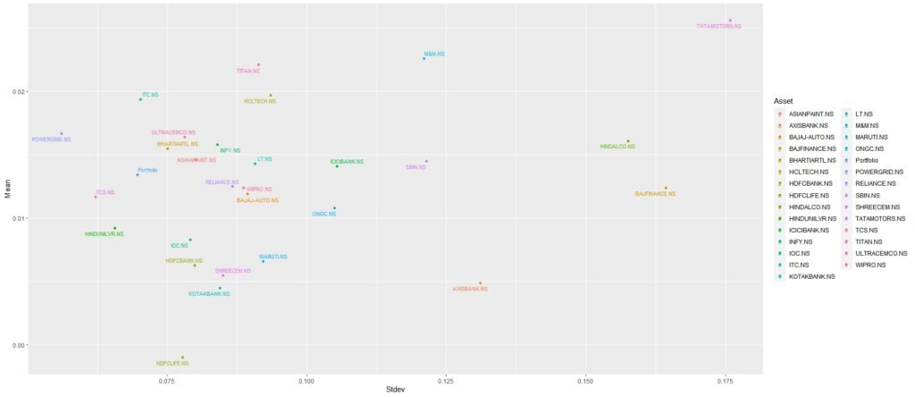
Investment decisions often involve constructing portfolios with diverse assets, each contributing a specific weight to the overall allocation. To simulate and optimize such portfolios, analysts frequently require a set of weighted random values. In this article, we will guide you through the process of generating weighted random values in R for portfolio analysis. We will use a list of 30 prominent stocks from the Nifty 50 index as our example dataset. Also, read Portfolio Optimization using Markowitz’s Mean Variance Method in R Why Generate Weighted Random Values for Portfolio Analysis? Portfolio analysis is a critical aspect of investment management. It involves constructing a diversified portfolio of assets to achieve specific financial goals while managing risk. Generating weighted random values serves several purposes: Step-by-Step Guide to Generating Weighted Random Values in R: Step 1: Data Retrieval and Preparation To start, we collect historical price data for stocks from the Nifty 50 index using the tidyquant package in R. This dataset will serve as the basis for our portfolio analysis. Step 2: Generating Random Weights Next, we need to generate random weights for our 28 stocks, which will represent their allocations in the portfolio. We do this using the runif function in R, which generates random numbers between 0 and 1. Step 3: Creating the Weighted Portfolio We then use the tq_portfolio function to create our weighted portfolio. This function combines the returns of the assets based on the weights we’ve generated, effectively simulating a portfolio. Step 4: Analyzing Portfolio Performance Now that we have our weighted portfolio, we can analyze its performance. We calculate key metrics such as standard deviation (risk) and mean return. Step 5: Visualization To gain insights from our portfolio, we visualize the relationship between risk (standard deviation) and expected returns. For more such Projects in R, Follow us at Github/quantifiedtrader Conclusion Generating weighted random values is a fundamental step in portfolio analysis and optimization. It enables investors and analysts to explore different portfolio scenarios and make informed investment decisions. By following this step-by-step guide in R, you can simulate and analyze portfolios, helping you to better understand the dynamics of your investments and ultimately make more informed choices in the world of finance. FAQs Q1: What is portfolio analysis in finance? Portfolio analysis is a process of evaluating and managing a collection of investments, known as a portfolio, to achieve specific financial goals while balancing risk. Q2: Why is portfolio analysis important? Portfolio analysis helps investors make informed decisions by assessing the performance, risk, and diversification of their investments. Q3: What are weighted random values in portfolio analysis? Weighted random values are randomly generated weights assigned to assets in a portfolio. They simulate different asset allocations for analysis. Q4: How can I generate weighted random values in R? You can generate weighted random values in R by using the runif function to create random weights and normalize them to sum up to 1. Q5: What is the standard deviation in portfolio analysis? Standard deviation measures the volatility or risk of a portfolio. A lower standard deviation indicates lower risk.

Optimizing Investment using Portfolio Analysis in R Read More »

Portfolio Optimization using Markowitz's Mean Variance Method

Portfolio Optimization using Markowitz’s Mean Variance Method in R

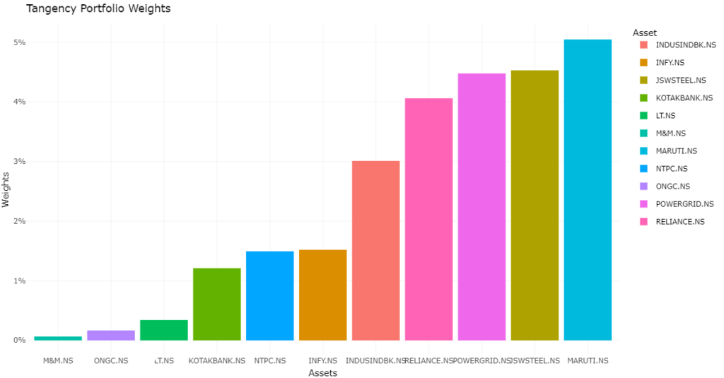
In the world of finance, investors are perpetually seeking the golden balance between maximizing returns and minimizing risk. The Markowitz Model, developed by Nobel laureate Harry Markowitz in 1952, revolutionized modern portfolio optimization theory by introducing the concept of diversification and risk management. At the core of this theory lie two key portfolios: the Minimum Variance Portfolio and the Tangency Portfolio, which form the basis of the Efficient Frontier. In this article, we will explore these essential concepts, provide the mathematical equations behind them, and guide you through their practical implementation using R programming. For more such Projects in R, Follow us at Github/quantifiedtrader Understanding the Markowitz Model The Markowitz Model is built upon the fundamental principle that diversification can lead to portfolio optimization and a more favorable risk-return tradeoff. It introduced the concept of risk as variance, quantifying it in terms of portfolio volatility. Here’s how the key elements of this model work together: Equations Behind Markowitz’s Model To calculate the Minimum Variance Portfolio and Tangency Portfolio, you need the following equations: Minimum Variance Portfolio (MVP): Tangency Portfolio: Practical Implementation with R Now, let’s put the theory into practice with R programming. The provided code demonstrates how to calculate these portfolios and visualize the Efficient Frontier using historical stock data. This code utilizes the quantmod and ggplot2 libraries to retrieve historical stock data, calculate portfolio returns and risk, and visualize the results. You can adapt this code to your own dataset and customize it as needed. Conclusion The Markowitz Model, with its Minimum Variance and Tangency Portfolios, remains a cornerstone of modern portfolio theory. By understanding and implementing these concepts, investors can better navigate the complex world of finance, optimizing their portfolios to achieve their financial goals while managing risk effectively. Whether you’re a seasoned investor or a beginner, Markowitz’s ideas continue to offer valuable insights into the art of portfolio management. FAQs Why is diversification important in the Markowitz Model? Diversification spreads risk across different assets, reducing the overall portfolio risk. Markowitz’s model quantifies this diversification benefit and helps investors optimize their portfolios accordingly. What is the Sharpe Ratio, and why is it significant? The Sharpe Ratio measures the risk-adjusted return of a portfolio. It’s essential because it helps investors evaluate whether the excess return they earn is worth the additional risk taken. Can I apply the Markowitz Model to any asset class? Yes, you can apply the Markowitz Model to any set of assets, including stocks, bonds, real estate, or a combination of asset classes. However, accurate historical data and covariance estimates are crucial for its effectiveness.

Portfolio Optimization using Markowitz’s Mean Variance Method in R Read More »

Scroll to Top