Analyzing Portfolio Downside Risk with R

In the world of finance and investment, understanding the risk associated with your portfolio is paramount. One key aspect of risk analysis is examining downside risk, which refers to the potential for unfavorable returns or extreme losses. This is also termed as the Portfolio downside risk analysis.

In this article, we will walk you through a comprehensive analysis of your portfolio’s downside risk using R, a powerful programming language for data analysis. We will explore essential statistical concepts such as kurtosis and skewness to gain insights into how your portfolio’s risk has evolved over time.

Also, read Optimizing Investment using Portfolio Analysis in R

What is Kurtosis?

Kurtosis is a statistical measure that describes the distribution of returns in a portfolio. It measures the “tailedness” of the distribution, indicating whether the data has heavy tails or light tails compared to a normal distribution. Kurtosis helps investors assess the risk associated with extreme returns.

The formula for kurtosis (K) is as follows:

Where:

• xi​ represents each individual return in the portfolio.
• ˉxˉ is the mean (average) return of the portfolio.
• σ is the standard deviation of the portfolio returns.
• n is the number of observations (months, in most cases).

Interpreting Kurtosis

1. Leptokurtic (K > 3): A leptokurtic distribution has heavy tails, indicating a higher probability of extreme returns. This suggests that the portfolio has a higher risk of significant gains or losses.
2. Mesokurtic (K = 3): A mesokurtic distribution has tails similar to a normal distribution. It implies that the portfolio’s returns are consistent with the expectations of a normal distribution.
3. Platykurtic (K < 3): A platykurtic distribution has light tails, meaning there is a lower likelihood of extreme returns. This indicates a lower risk compared to a leptokurtic distribution.

What is Skewness?

Skewness measures the asymmetry of the distribution of returns in a portfolio. It helps investors understand whether the portfolio is more likely to experience positive or negative returns and the degree of asymmetry.

The formula for skewness (S) is as follows:

Where the variables are the same as in the kurtosis formula.

Interpreting Skewness

1. Positive Skew (S > 0): A positively skewed distribution means that the portfolio is more likely to experience extremely positive returns. It has a longer right tail, indicating a potential for large gains.
2. Negative Skew (S < 0): A negatively skewed distribution suggests that the portfolio is more likely to experience extreme negative returns. It has a longer left tail, signaling a potential for significant losses.
3. Symmetric (S = 0): A skewness of zero implies that the distribution is symmetric, and the likelihood of positive and negative returns is balanced.

How to calculate Portfolio Downside Risk, Kurtosis and skewness using R

Step 1: Load the Necessary Packages

# Core
library(tidyverse)
library(tidyquant)

To begin, we load the essential R packages, including tidyverse and tidyquant, which provides a wide range of tools for data manipulation and financial analysis.

Step 2: Define Your Portfolio and time frame

# Choose your stocks and define the time period
symbols <- c("CIPLA.NS", "MARUTI.NS", "SBIN.NS","RELIANCE.NS")
start_date <- "2017-01-01"
end_date <- "2023-08-01"

Select the stocks you want to include in your portfolio and specify the start and end dates for your analysis.

Step 3: Import Stock Prices

# Import historical stock prices
prices <- tq_get(x = symbols, 
                get = "stock.prices",
                from = start_date, 
                to = end_date)

Retrieve historical stock price data for the chosen stocks within the specified timeframe.

Step 4: Calculate Monthly Returns

# Calculate monthly returns
returns_tbl <- prices %>%
    group_by(symbol) %>%
    tq_transmute(select = adjusted, 
                 mutate_fun = periodReturn, 
                 period = "monthly",
                 type = "log") %>%
    slice(-1) %>%
    ungroup() %>%
    set_names(c("asset", "date", "returns"))

Compute monthly returns for each asset in your portfolio using a logarithmic transformation and Assign weights to each asset in your portfolio, reflecting the allocation of investments.

Step 5: Build the Portfolio and Assign Portfolio Weights

Construct the portfolio using the assigned weights, and ensure that returns are rebalanced on a monthly basis to simulate real-world scenarios.

# Define portfolio weights
portfolio_weights <- c(0.25, 0.25, 0.2, 0.2, 0.1)
# Build the portfolio
portfolio_returns_tbl <- returns_tbl %>%
    tq_portfolio(assets_col = asset, 
                 returns_col = returns, 
                 weights = portfolio_weights, 
                 rebalance_on = "months", 
                 col_rename = "returns")

Step 6: Compute Kurtosis and Rolling Kurtosis

Calculate the kurtosis of the portfolio’s returns, a measure that quantifies the risk associated with extreme values. Compute and visualize rolling kurtosis to observe changes in downside risk over time.

# Calculate portfolio kurtosis
portfolio_kurtosis <- portfolio_returns_tbl %>%
    tq_performance(Ra = returns, 
                   performance_fun = table.Stats) %>%
    select(Kurtosis)
    
# Define a rolling window size
window_size <- 24

# Calculate rolling kurtosis
rolling_kurtosis_tbl <- portfolio_returns_tbl %>%
    tq_mutate(select = returns, 
              mutate_fun = rollapply,
              width = window_size,
              FUN = kurtosis, 
              col_rename = "kurt") %>%
    na.omit() %>%
    select(-returns)

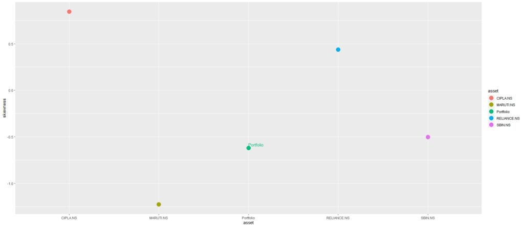
Step 7: Analyze Skewness and Return Distributions

Calculate the skewness of individual assets and the portfolio, and visualize the distribution of returns for each asset.

# Calculate asset skewness
asset_skewness_tbl <- returns_tbl %>%
    group_by(asset) %>%
    summarise(skew = skewness(returns)) %>%
    ungroup() %>%
    add_row(tibble(asset = "Portfolio",
                   skew = skewness(portfolio_returns_tbl$returns)))

# Plot skewness
# (Omitted for brevity)

# Plot distribution of returns
# (Omitted for brevity)

Now, let’s delve into the meaning of the terms and the insights we’ve gained:

Kurtosis: Kurtosis measures the distribution of returns. A higher kurtosis indicates a riskier distribution with the potential for extreme returns, both positive and negative. If the portfolio kurtosis is greater than 3, it suggests a higher risk of extreme returns. A positive portfolio skewness indicates a potential for positive outliers, while a negative skewness suggests a higher likelihood of negative outliers.

Rolling Kurtosis: This plot shows how the downside risk of the portfolio has changed over time. Peaks indicate periods of increased risk.

Skewness: Skewness assesses the symmetry of return distributions. Negative skewness suggests more downside risk, while positive skewness indicates more upside potential.

We observed that the portfolio’s downside risk improved slightly over the past year. During the pandemic, the portfolio experienced a surge in kurtosis, indicating high risk. However, recent data shows a negatively skewed distribution with lower kurtosis, signaling reduced risk. While historical data showed unattractive prospects, the portfolio now offers more consistent returns.

For more such Projects in R, Follow us at Github/quantifiedtrader

What does higher portfolio kurtosis mean?

When the portfolio kurtosis is higher, it means that the distribution of returns in the portfolio has heavier tails compared to a normal distribution. In other words, the portfolio has a higher probability of experiencing extreme returns, both positive and negative.

Here’s what a higher portfolio kurtosis implies:

1. Higher Risk: A higher kurtosis indicates that the portfolio carries a greater risk of extreme outcomes. There is an increased likelihood of experiencing significant gains or losses in a short period.
2. Volatility: The portfolio is more volatile and can exhibit rapid and substantial price fluctuations. This can make it riskier for investors, as they need to be prepared for potentially large and unexpected moves in the portfolio’s value.
3. Fat Tails: The distribution of returns has fatter tails, meaning that there is a higher chance of observing returns far from the mean (average). This can be a concern for investors seeking stability and predictability in their investments.
4. Diversification Impact: Higher kurtosis may indicate that diversification across assets in the portfolio might not be effectively reducing risk, as extreme events can still impact multiple assets simultaneously.

A higher portfolio kurtosis suggests that the portfolio’s returns are more volatile and that investors should be cautious about the potential for extreme outcomes, both positive and negative. It often indicates a higher level of risk associated with the investment.

what does higher portfolio skewness mean?

A higher portfolio skewness means that the distribution of returns in the portfolio is skewed towards one side of the mean (average). Specifically:

1. Positive Skewness: If the portfolio has positive skewness, it implies that the majority of returns tend to be concentrated on the left side of the mean, meaning there are more frequent small positive returns and fewer frequent large positive returns. This indicates a distribution with a “long tail” on the right side, where extreme positive returns can occur, but they are less common.
2. Negative Skewness: Conversely, if the portfolio has negative skewness, it suggests that the majority of returns are concentrated on the right side of the mean, with more frequent small negative returns and fewer frequent large negative returns. In this case, the distribution has a “long tail” on the left side, where extreme negative returns can occur, but they are less common.

Here’s what a higher portfolio skewness means:

• Risk Assessment: Positive skewness may indicate that the portfolio has a tendency for more frequent, but smaller, positive returns, potentially reflecting lower risk or a more conservative investment approach.
• Return Asymmetry: Negative skewness may indicate that the portfolio has a tendency for more frequent, but smaller, negative returns, which could be a concern for investors looking for more consistent and less risky returns.
• Impact on Investment Strategy: Understanding skewness is crucial for investors as it helps them assess the likelihood of experiencing extreme returns in either direction. It can influence investment decisions and risk management strategies.

A higher portfolio skewness provides insights into the distribution of returns and how they are skewed relative to the mean. Positive skewness suggests more frequent small positive returns, while negative skewness suggests more frequent small negative returns. Understanding skewness is valuable for investors in managing their portfolios and assessing potential risks and rewards.

Conclusion

Understanding and monitoring downside risk is essential for making informed investment decisions. Through R and statistical measures like kurtosis and skewness, you can gain valuable insights into your portfolio’s risk profile and make adjustments accordingly.